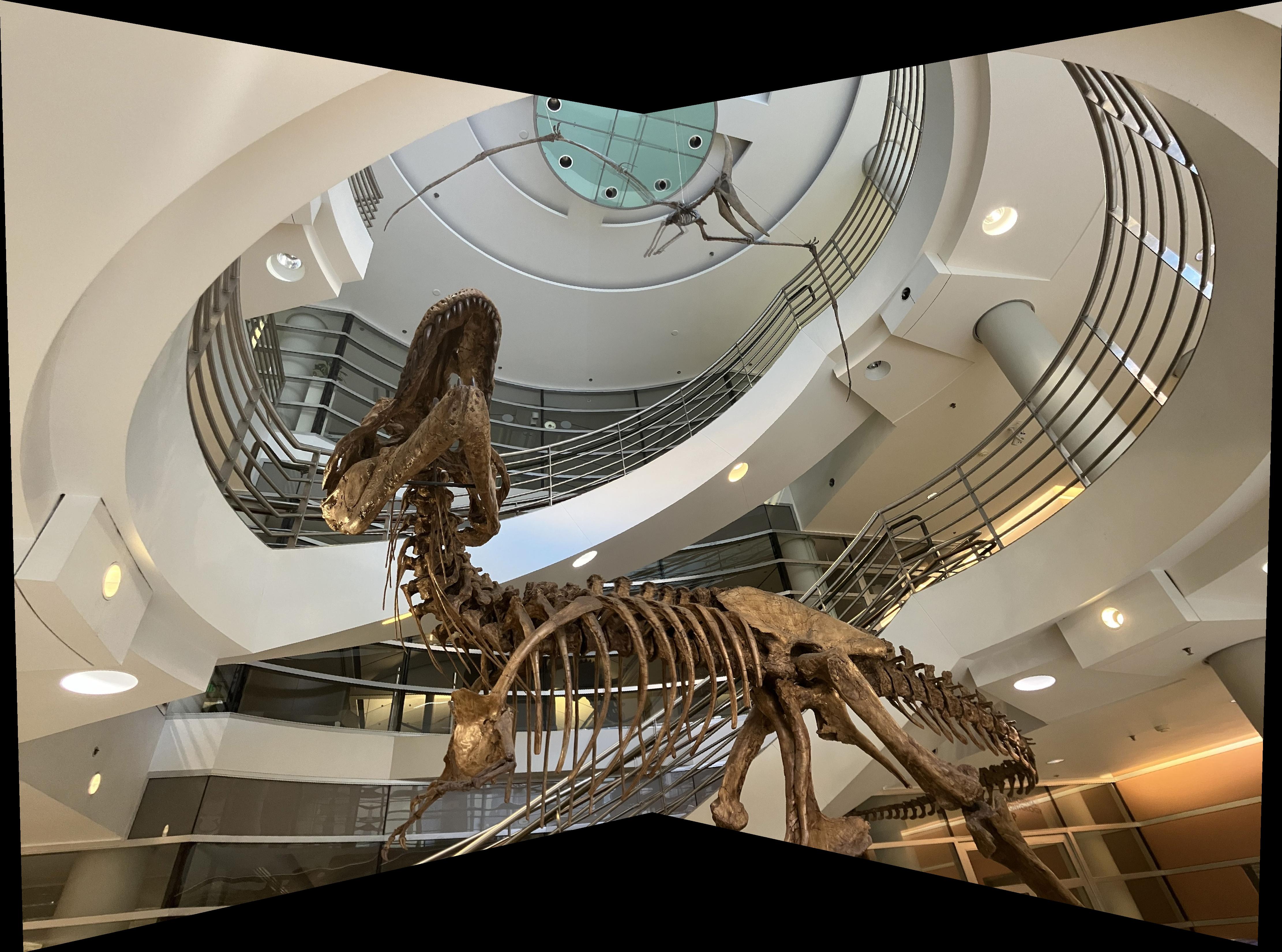
Overview
My goal for this project was to leverage image warping, registering, resampling, and compositing for visually interesting applications such as image rectification and image mosaics.
Section I: Shoot the Pictures
I took several pairs of images to stitch together and selected key points between shared features using the provided tool. To ensure that each image pair contained a projective transform, I fixed the center of projection while varying the camera angle.
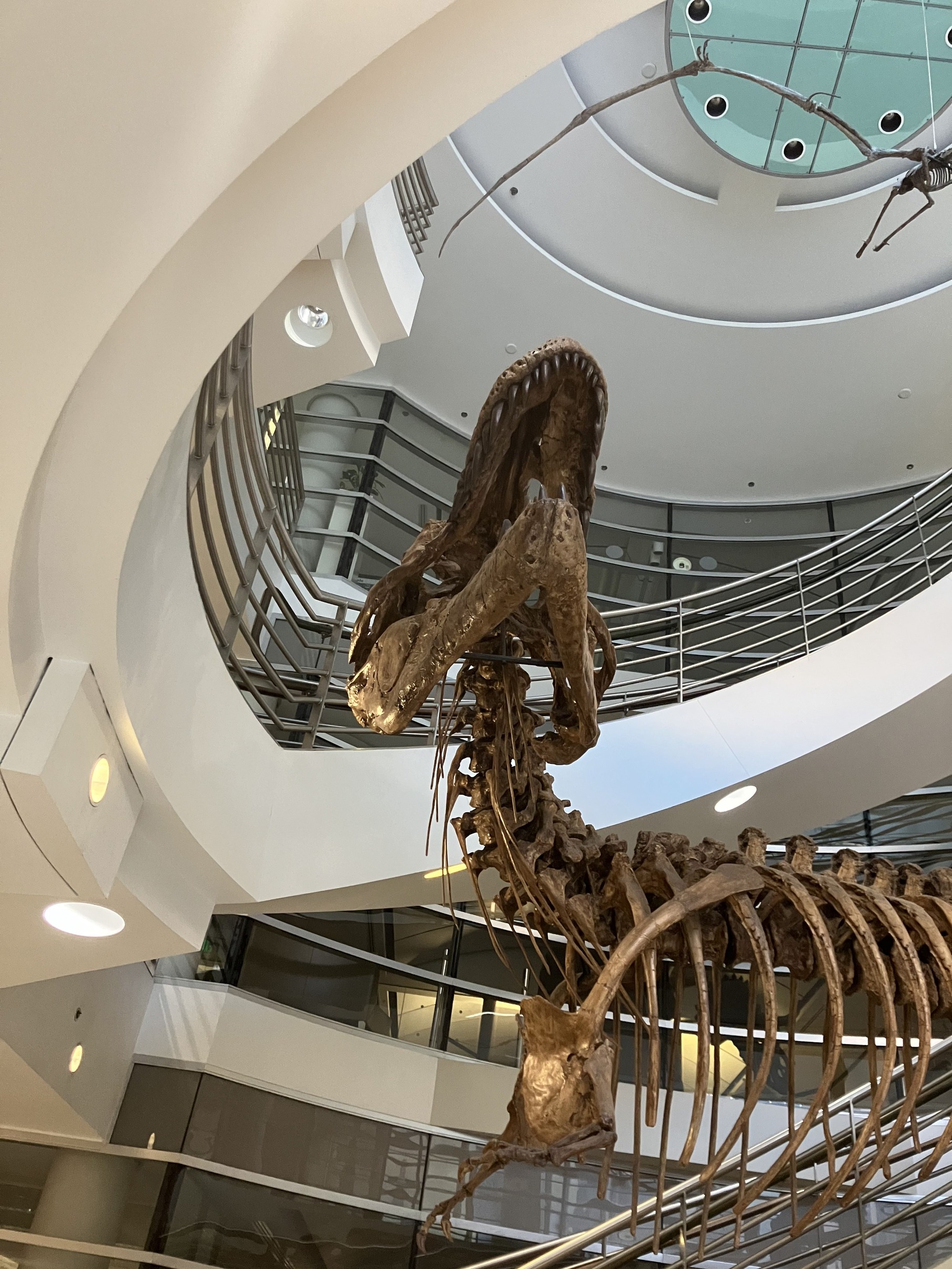
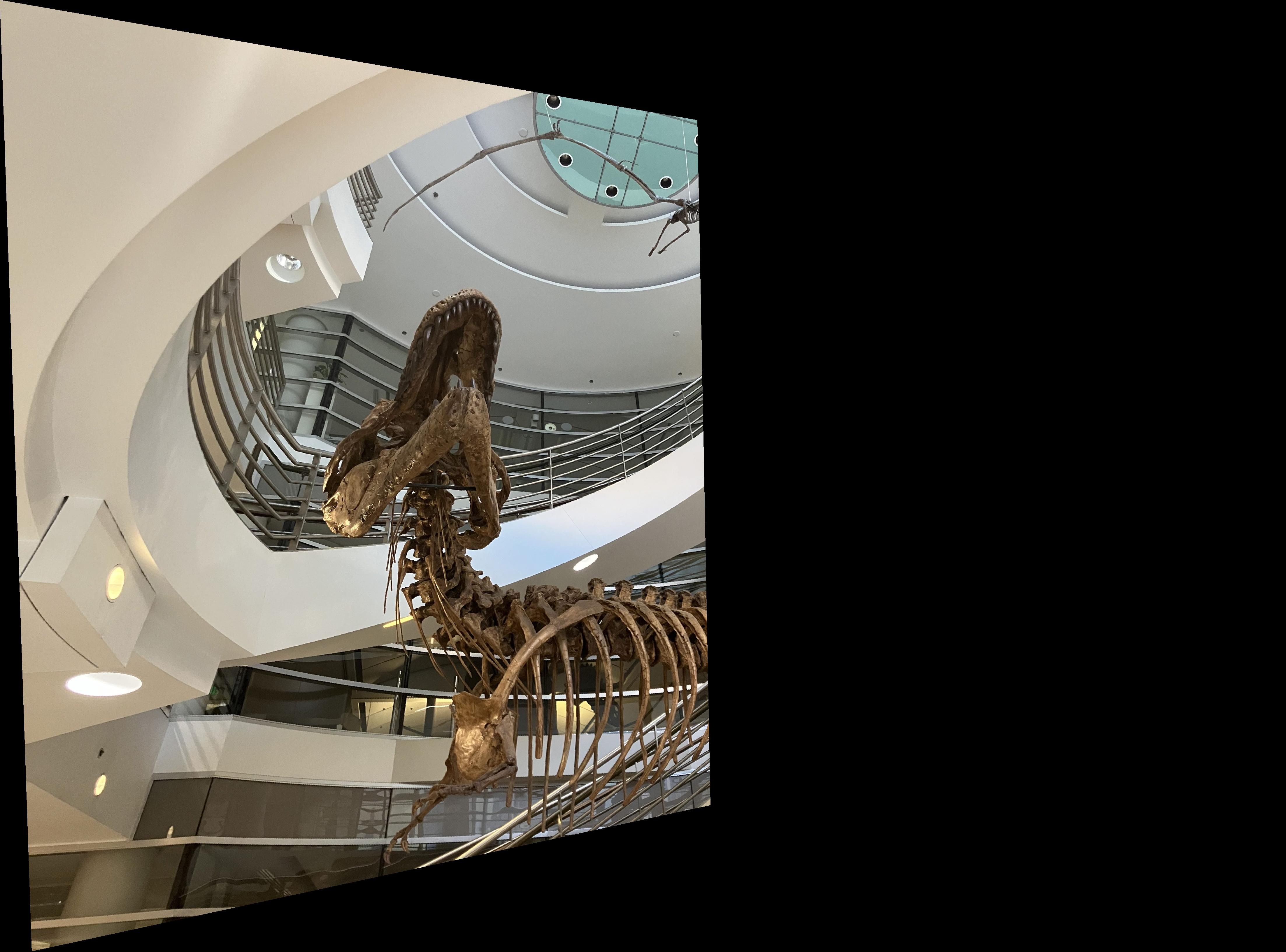
A T-Rex skeleton (left).
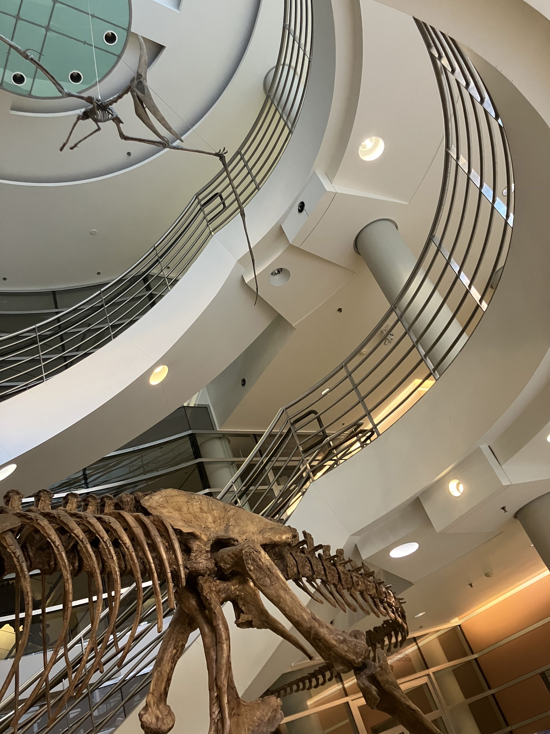
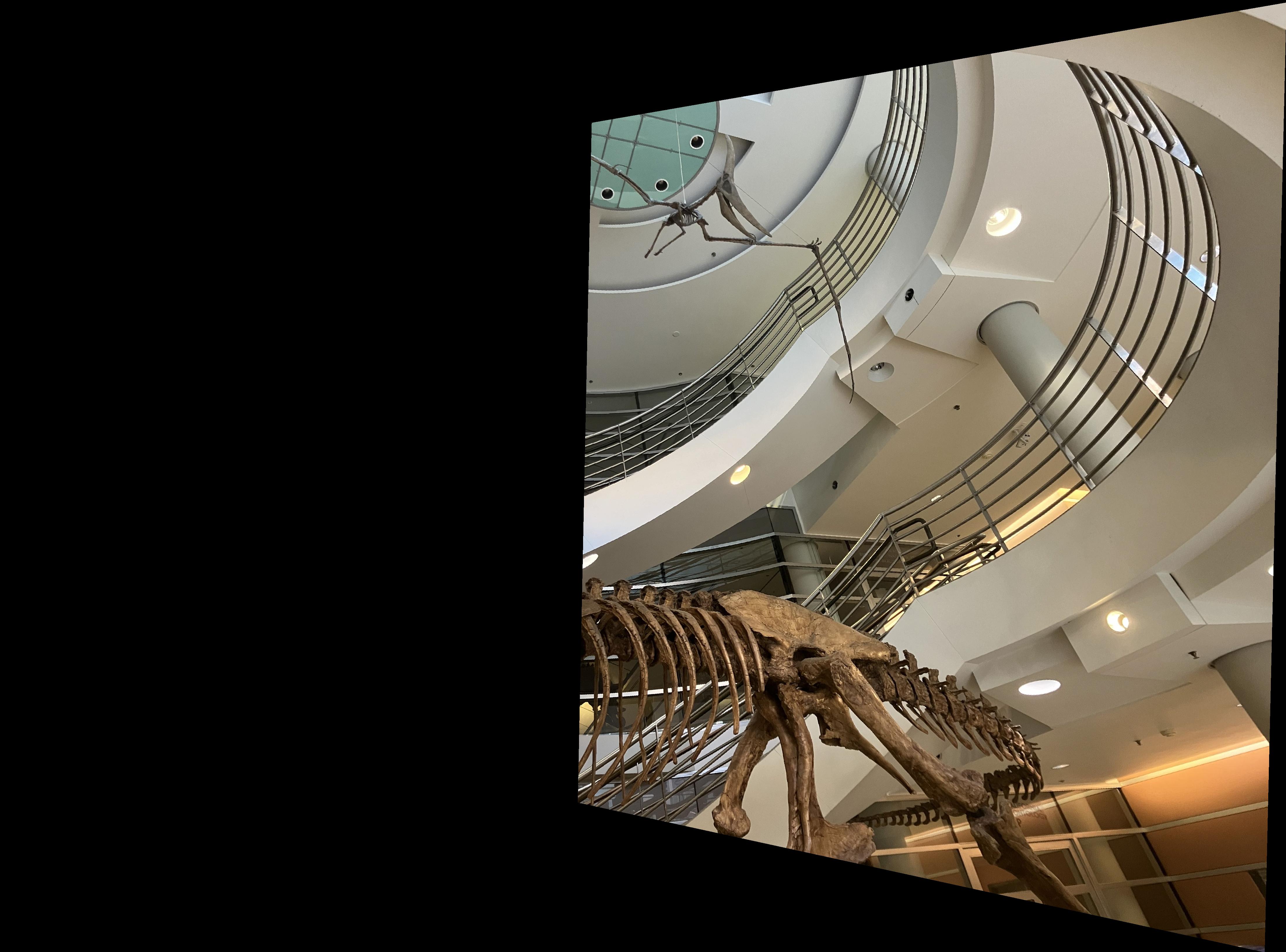
A T-Rex skeleton (right).
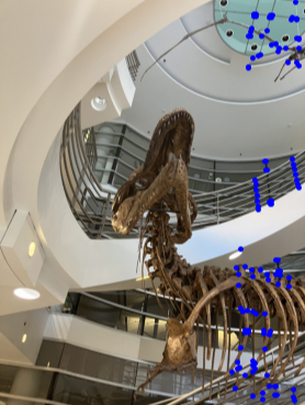
The correspondence points.
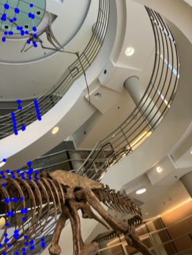
The correspondence points.

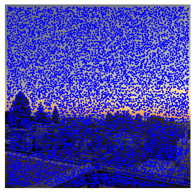
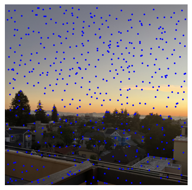
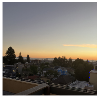
My balcony (left).

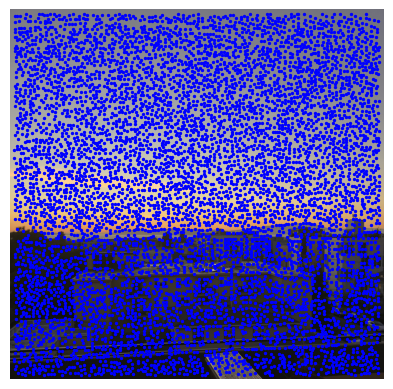
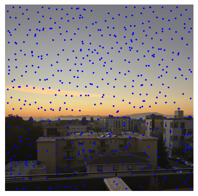
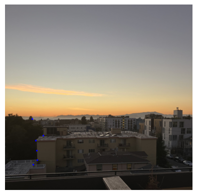
My balcony (right).
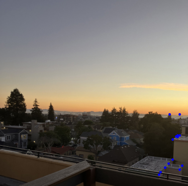
The correspondence points.
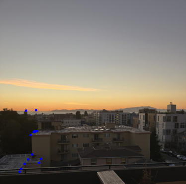
The correspondence points.
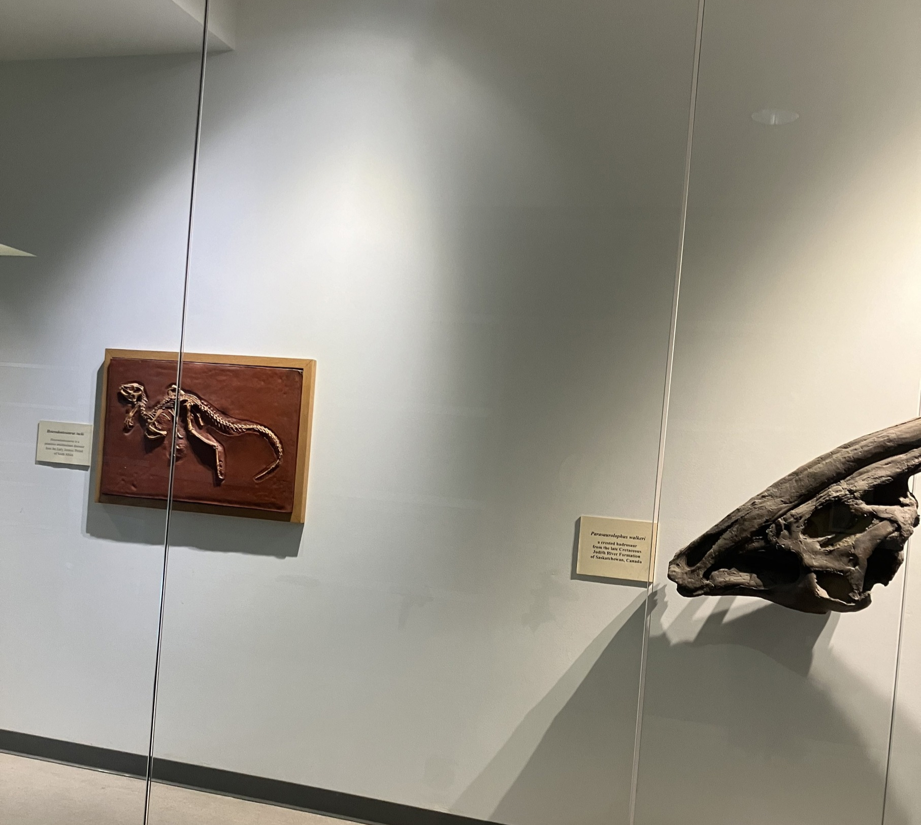
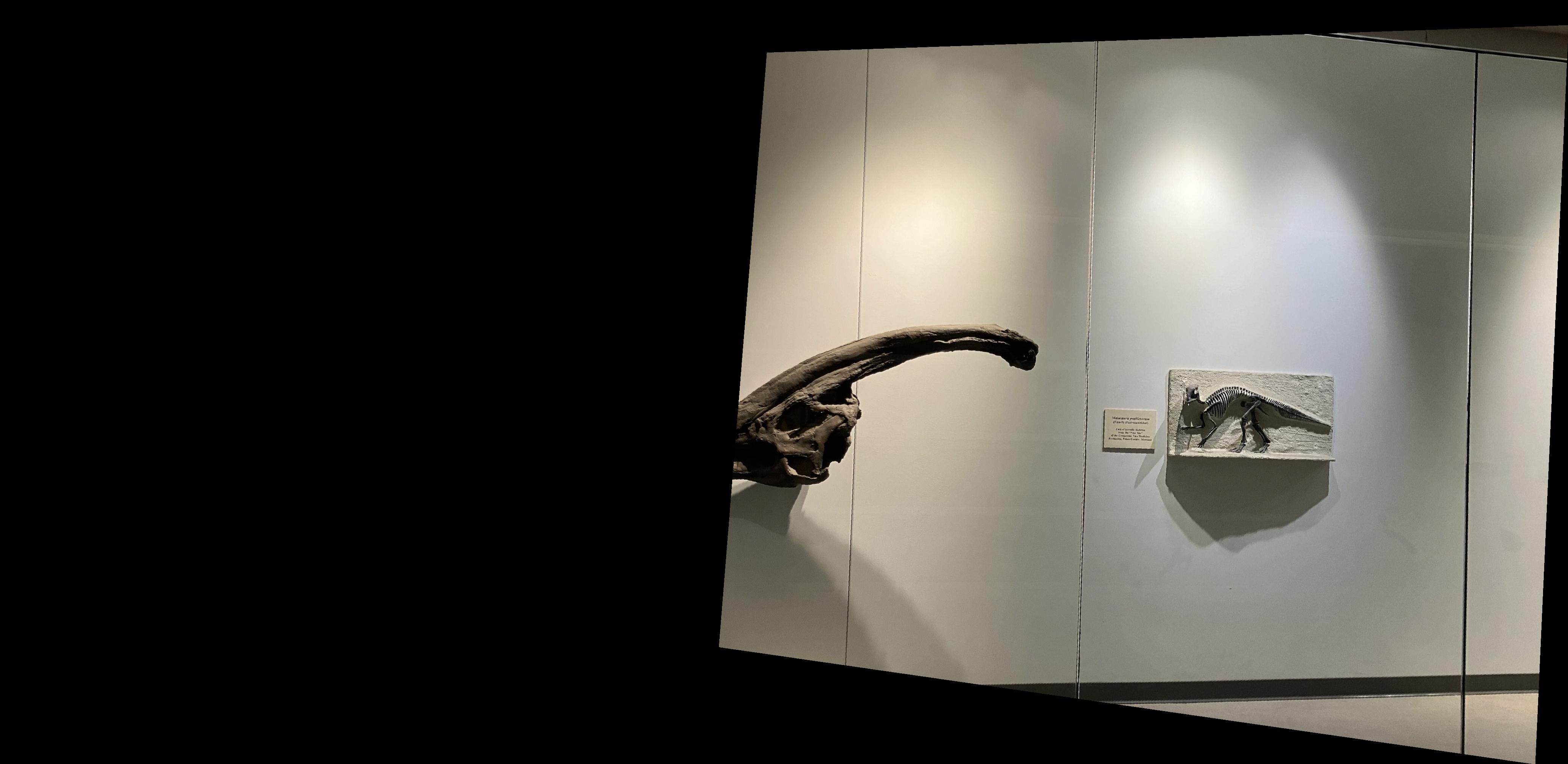
A Parasaurolophus skull (left).
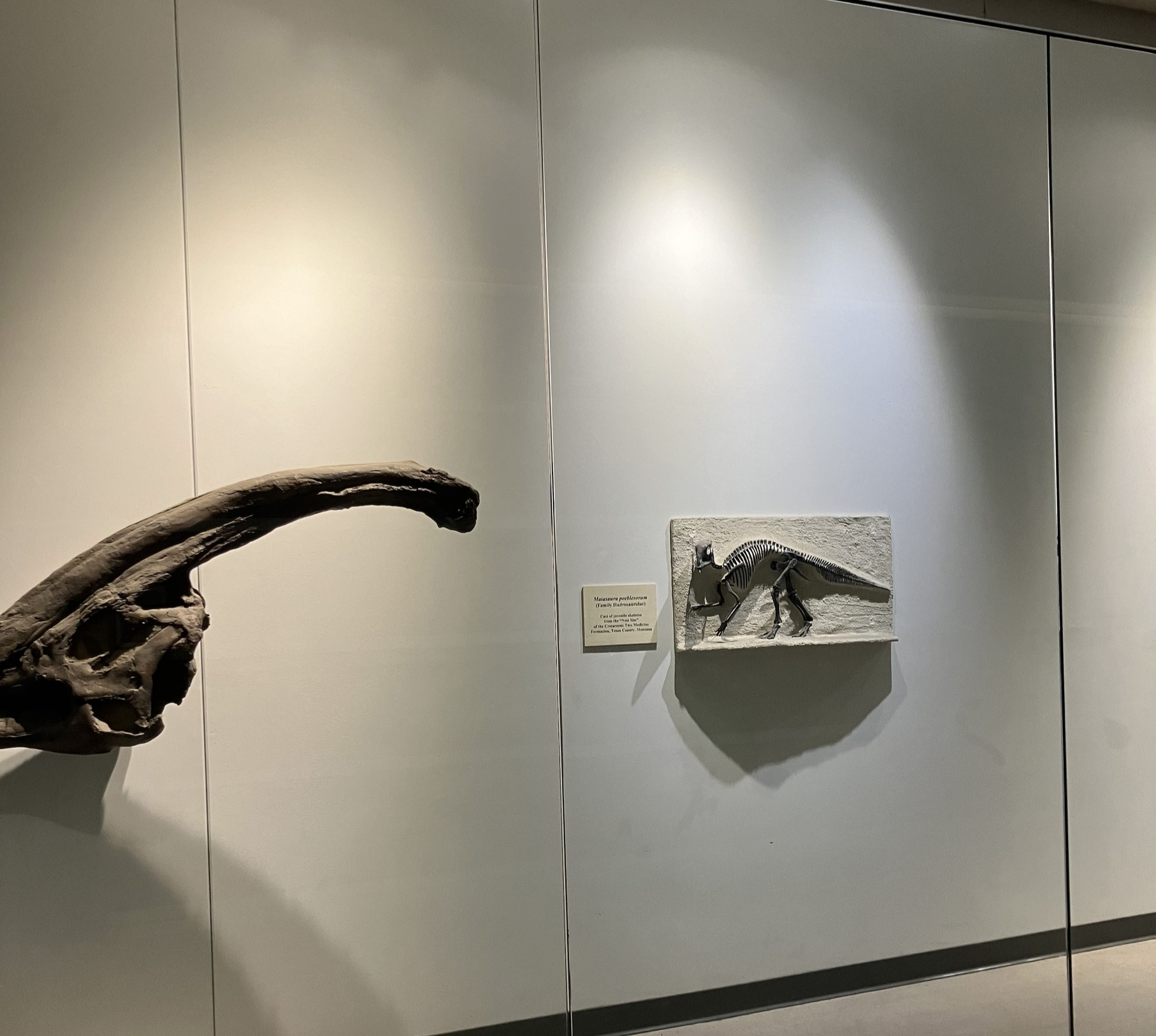
A Parasaurolophus skull (right).
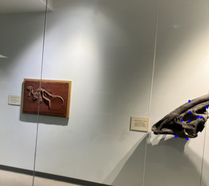
The correspondence points.
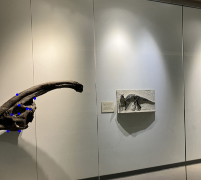
The correspondence points.
Section II: Recover Homographies
Given at least four sets of points from each, I can compute the homography between two images by finding the solution to the following system of equations:

The system can be solved as follows on the left. In the case that I’m using more than four sets of points, the system becomes overdetermined and can be solved using the least squares method on the right:

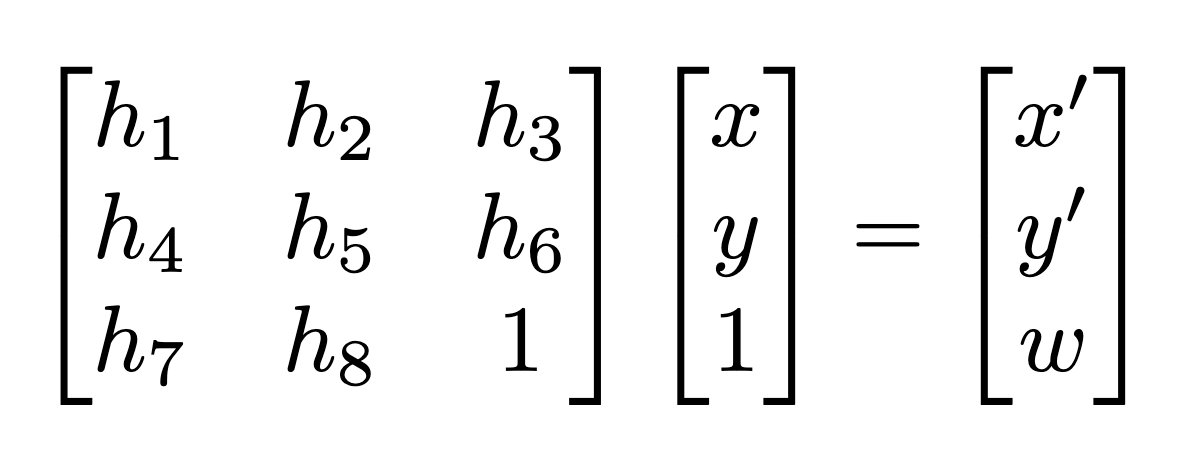
I can now construct the homography as the following 3x3 matrix using the obtained coefficients:
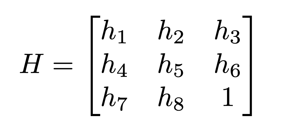
Finally, to warp the image, I apply the homography to homogenized sets of coordinates and scale the resulting coordinates by w :
Section III: Warp the Images
Image Rectification
To test my implementation, I rectified some images by mapping a warped surface to a flat rectangular plane. First, I selected key points at each corner of the surface I wanted to rectify, then calculated the homography from the source points to the points of the desired plane. To determine the bounds of the rectified image, I warped the bounds of the source image then found the mask contained by the bounds.
I performed inverse warping by using the inverse homography to map the mask back to the source image. Finally, I used nearest neighbor interpolation to populate the pixels of the rectified image based on the source image.
As you can see in the last result, this method doesn't always succeed in emulating real-life perspective.
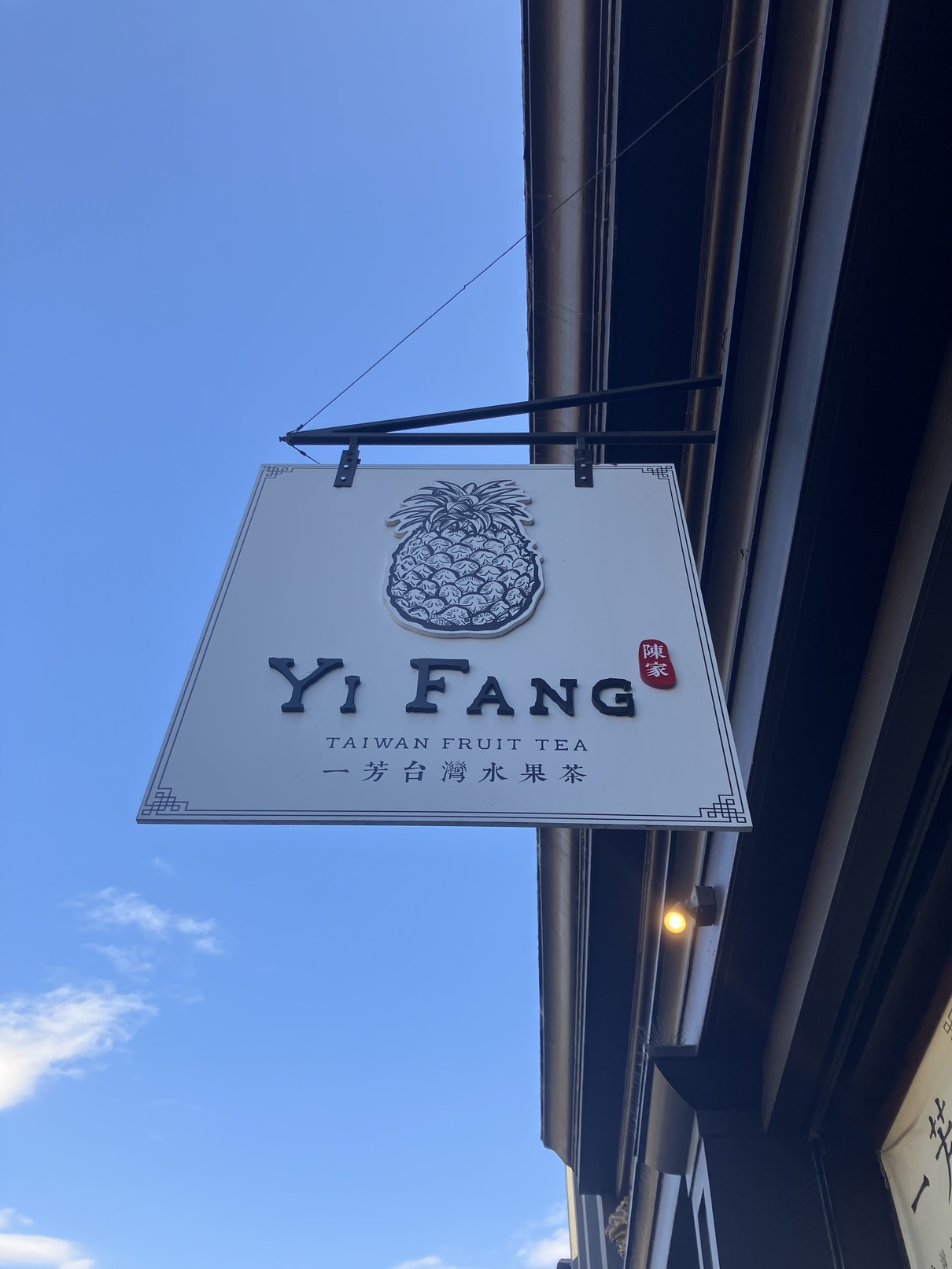
A Yi Fang sign.
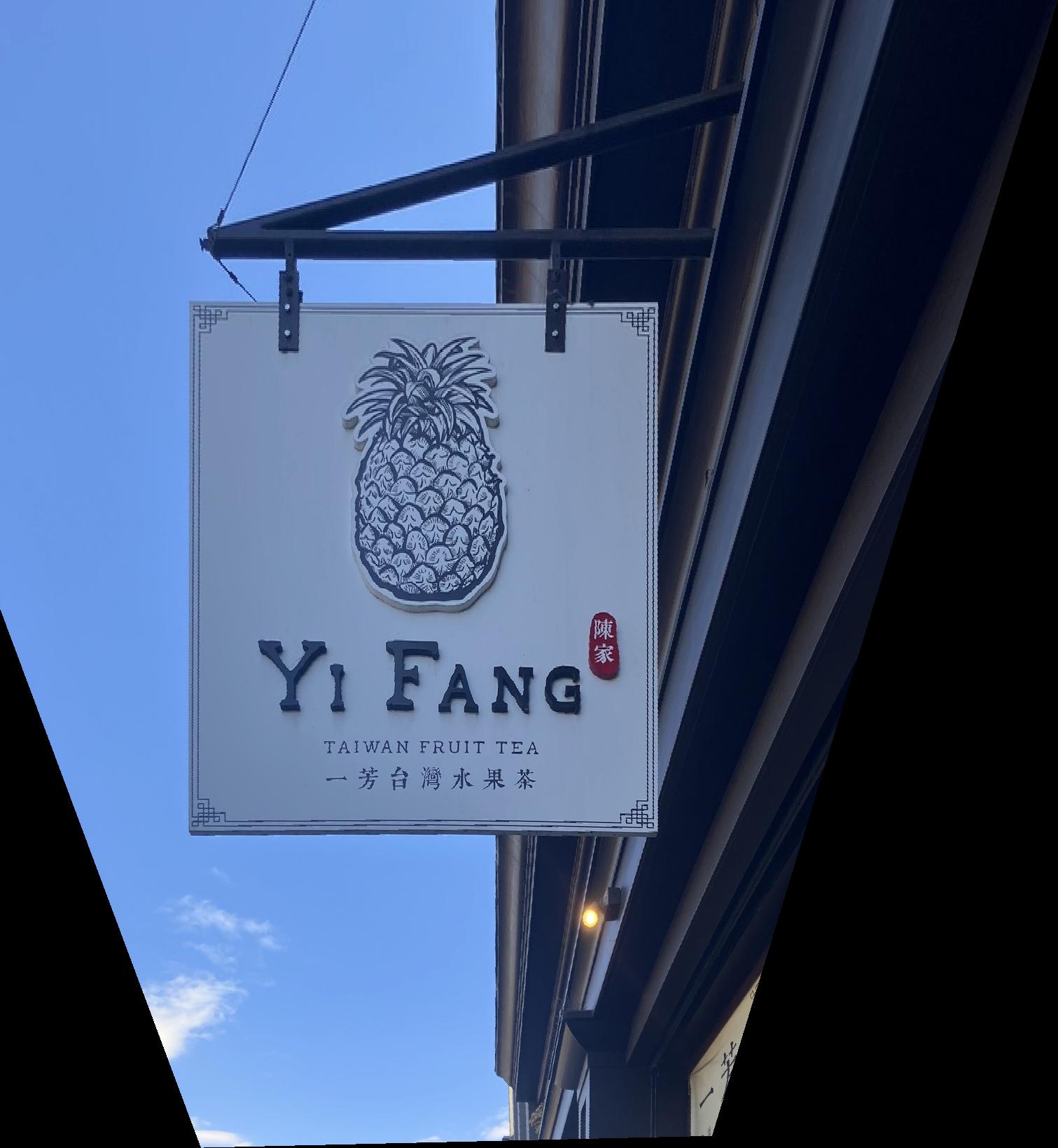
The rectified sign.
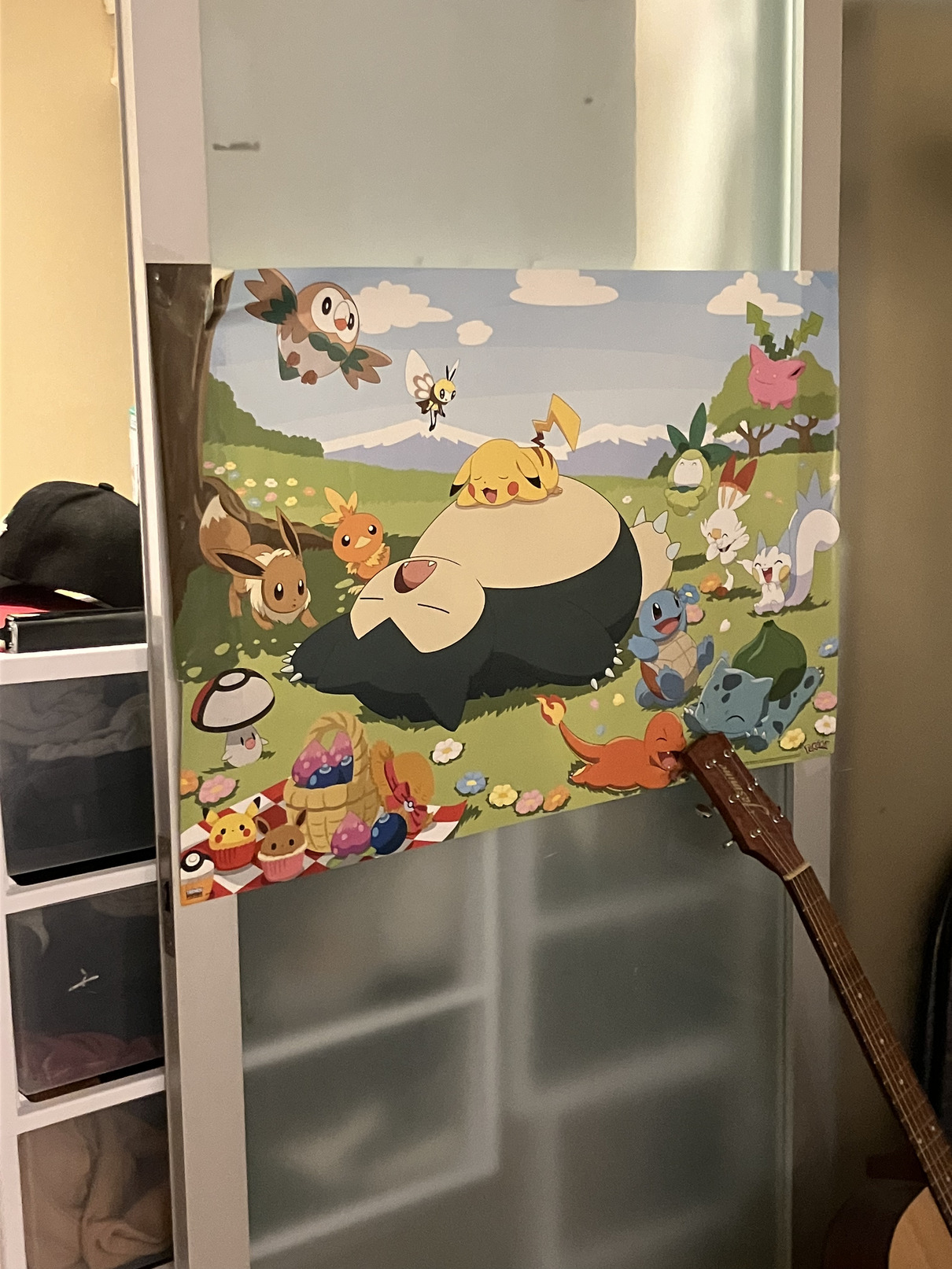
A Pokémon poster.
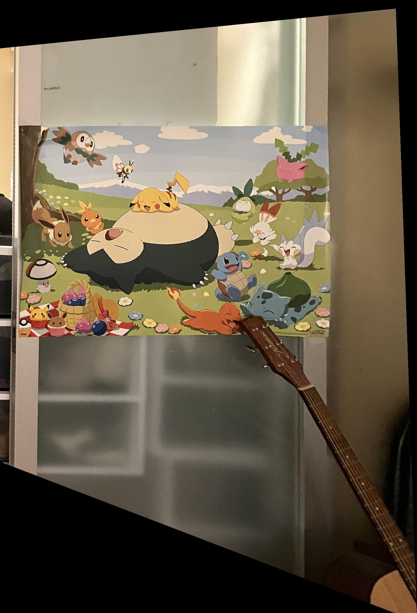
The rectified poster.
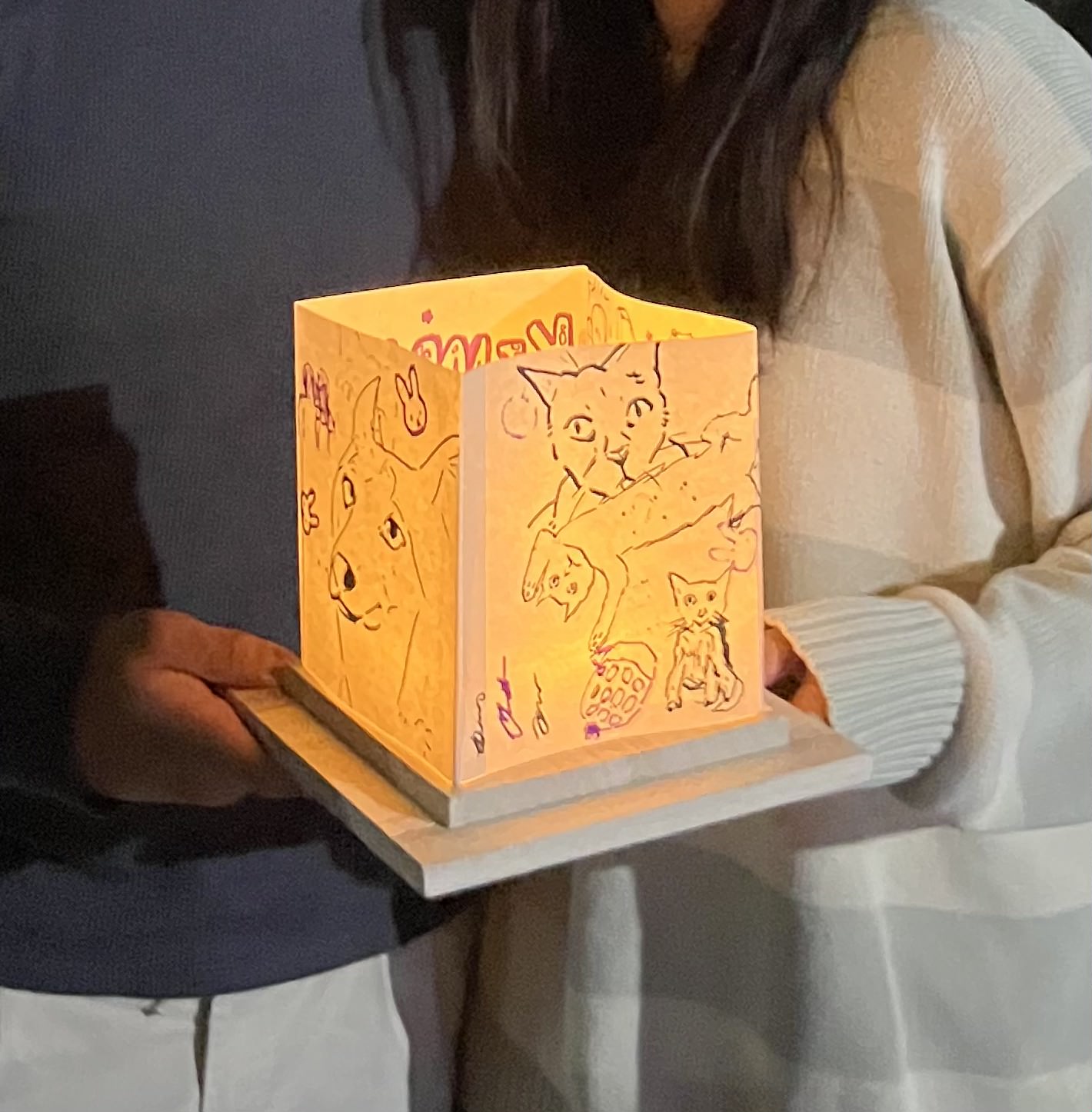
A lantern.
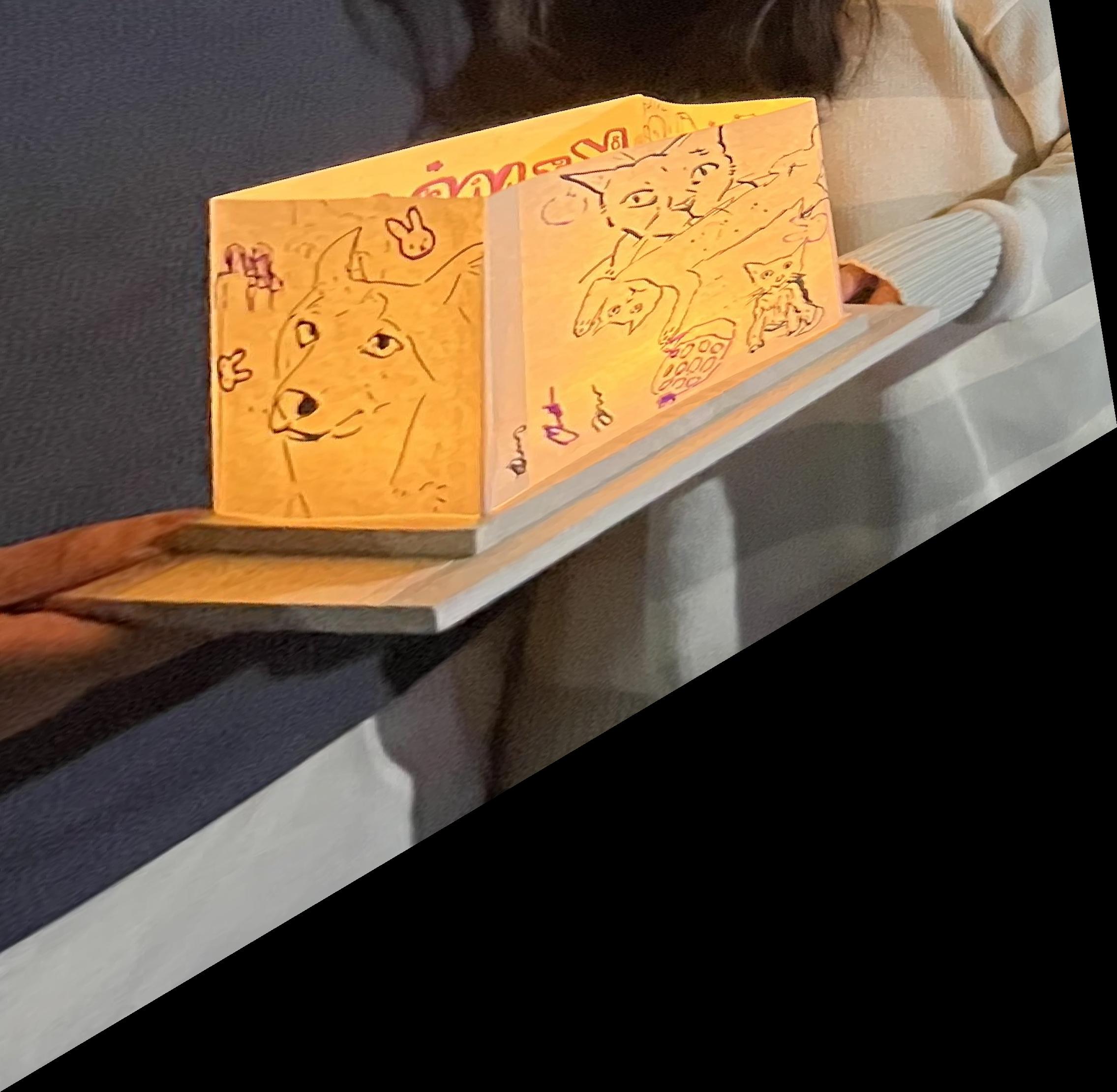
The "rectified" lantern.
Blend the Images Into a Mosaic
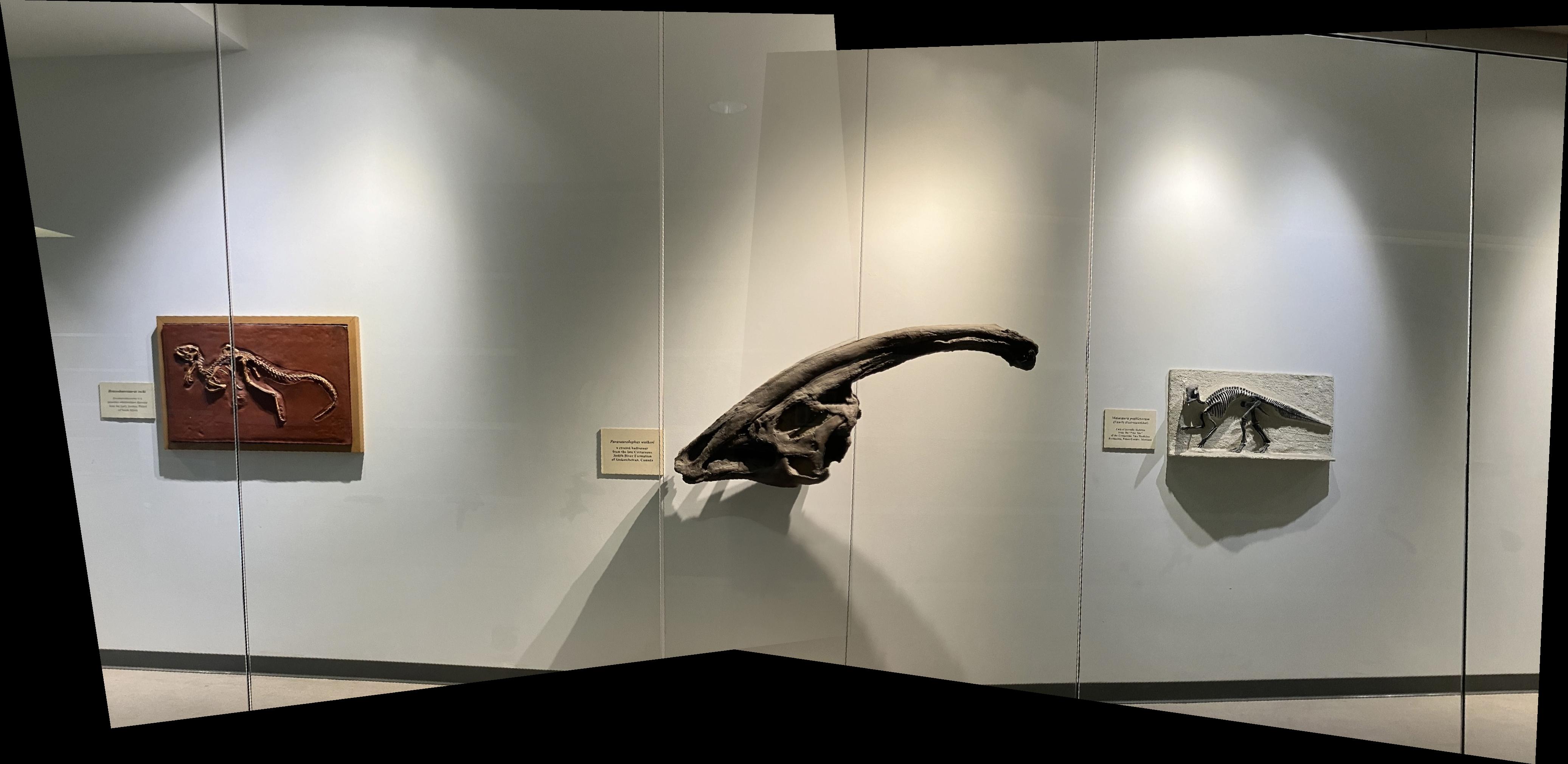
Finally, I moved onto blending images into a mosaic. Images in the mosaic must have the same perspective, so I averaged the key points of both images to find the target plane and computed the corresponding homographies to this plane.
I based the dimensions of the final bounding box on the sum of the minimum and maximum bounds of each image (post warp). To account for these new bounds, I shifted the warped images accordingly before placing them within the bounding box. The final mosaic is defined by the simple average between the alpha masks of both images. Highly intricate structures like the ribcage are still a bit blurry even after the warp, which could likely be improved by selecting more correspondence points.

The left image.
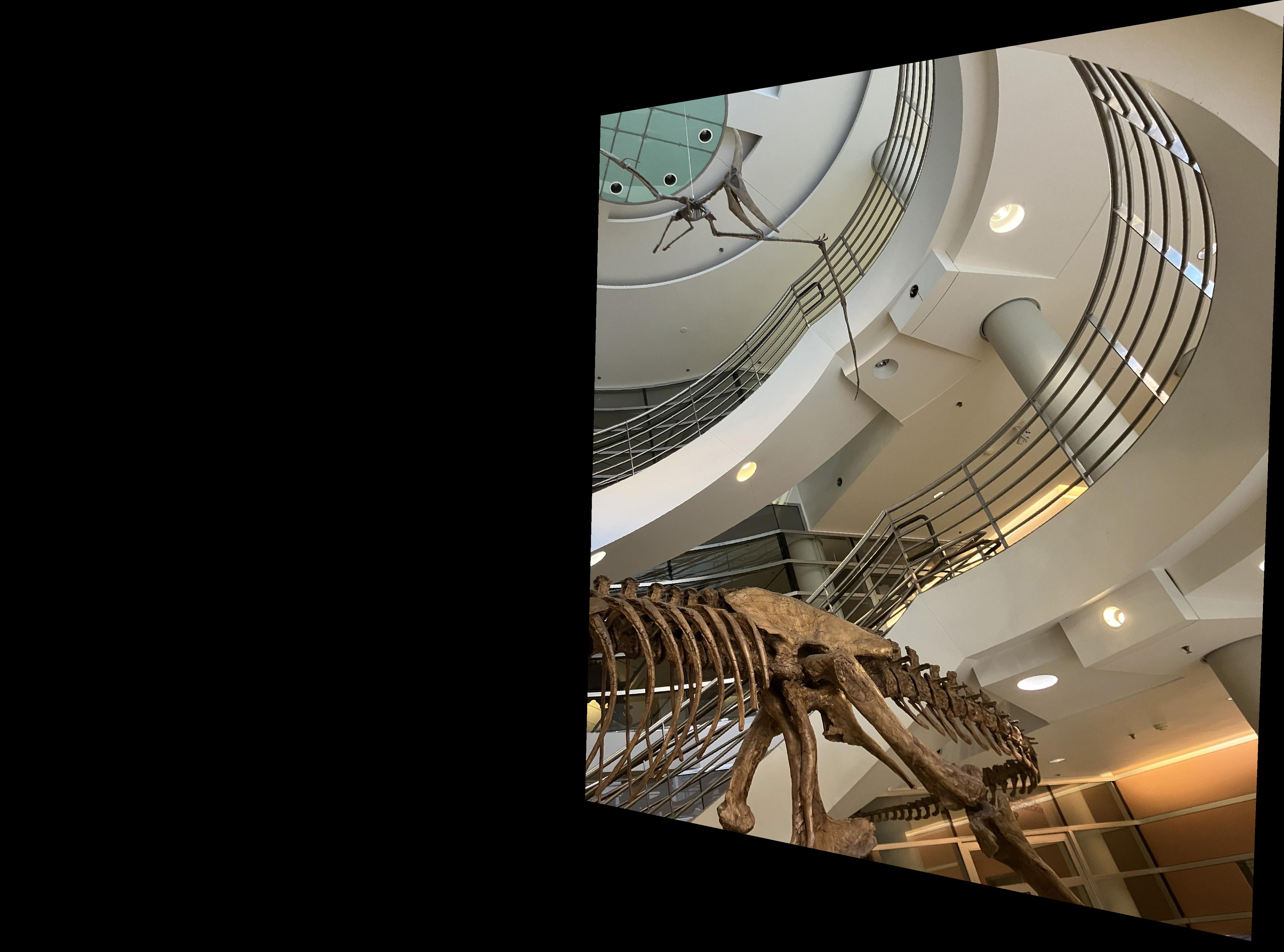
The right image.
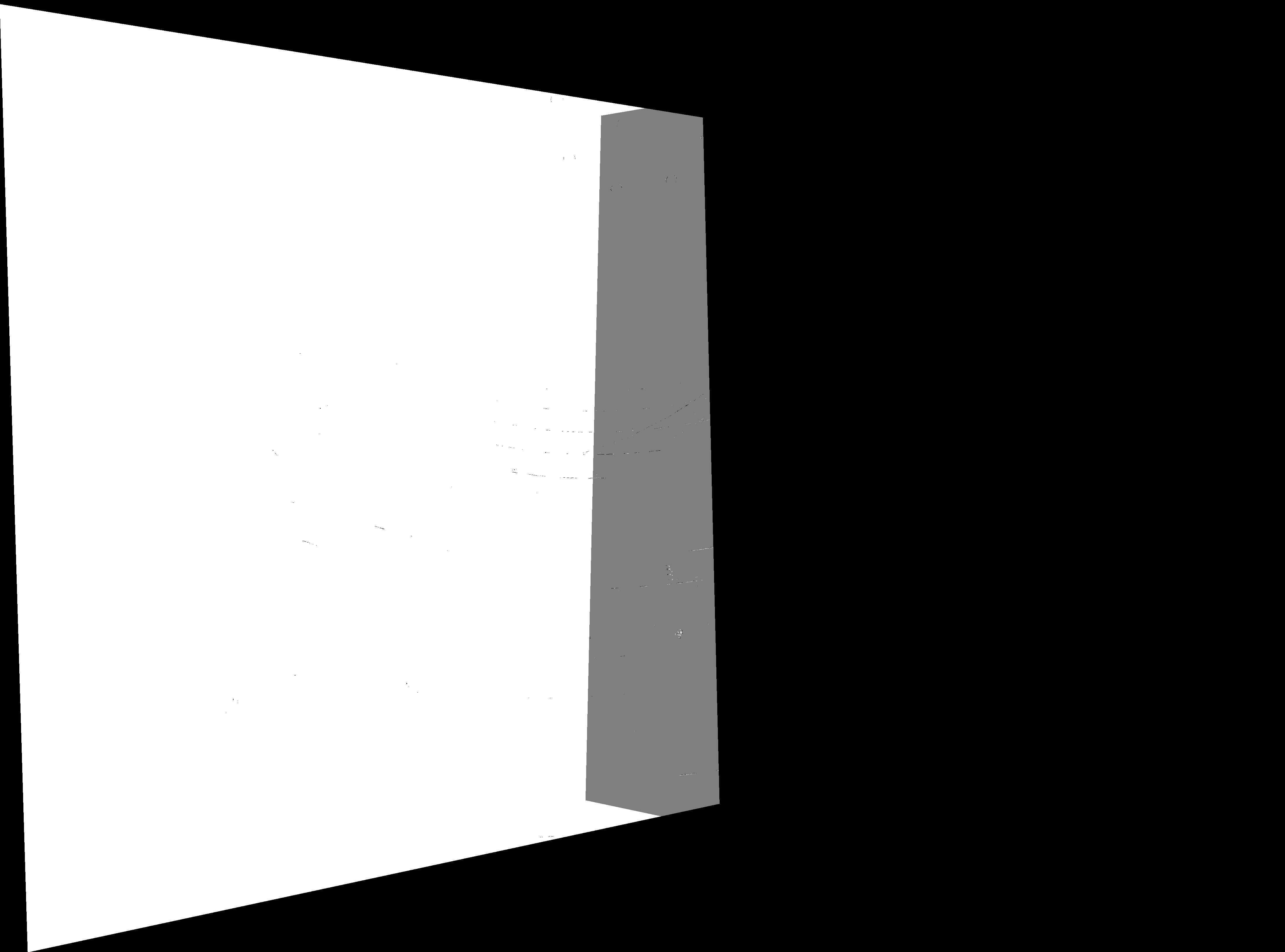
The left mask.
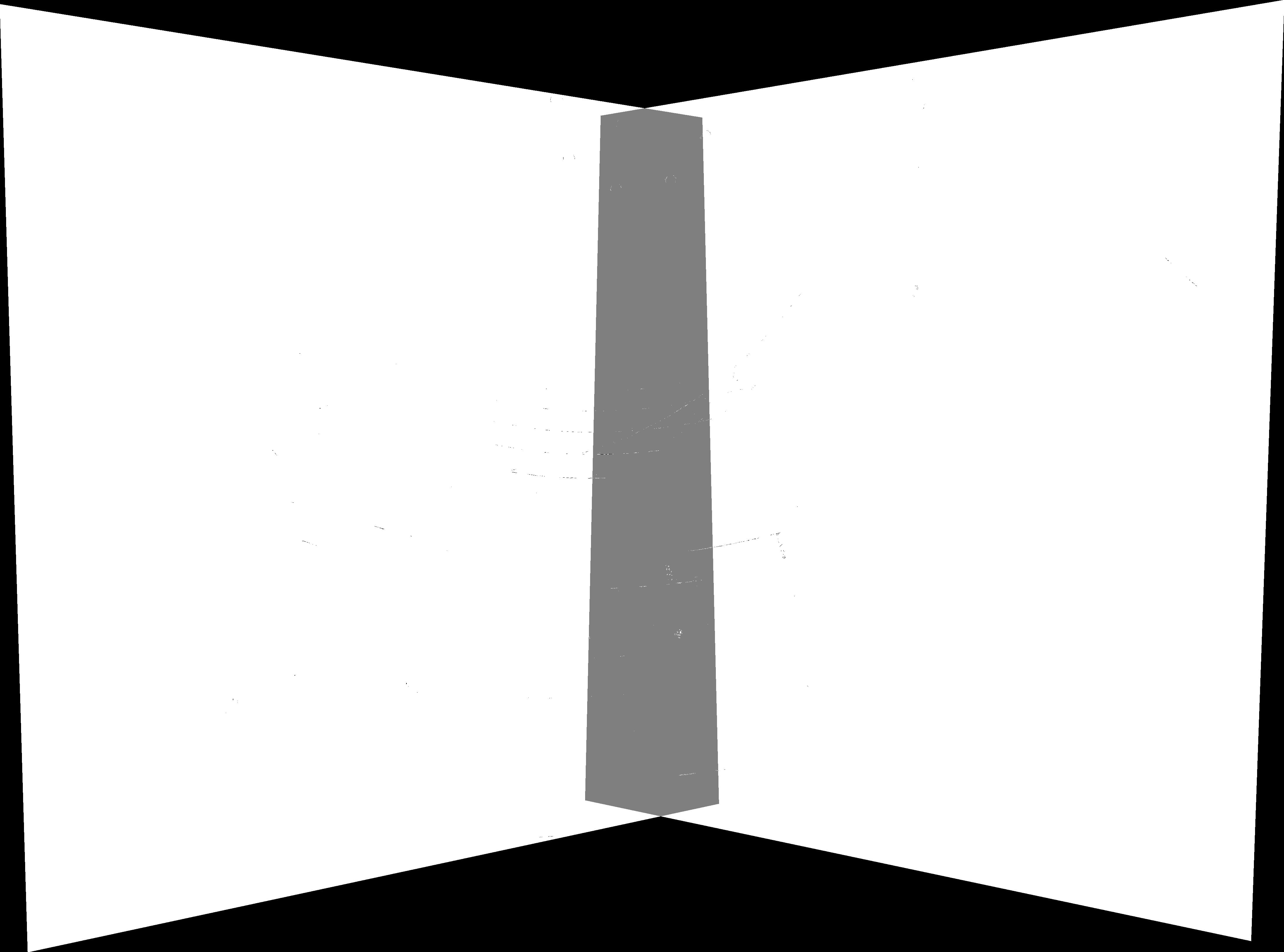
The combined mask.
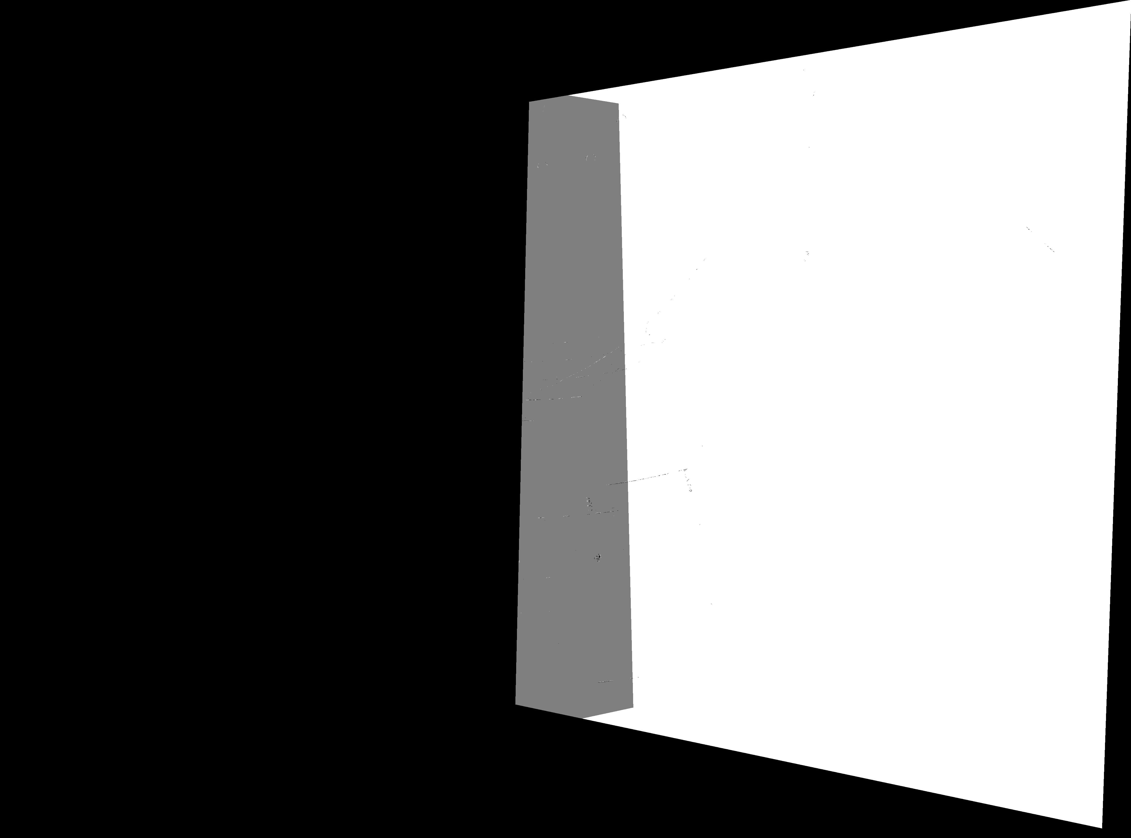
The right mask.

The final mosaic.
Due to differences in exposure between the images, the mask leaves a clear seam where the images overlap. I decided to "feather" my masks by having my left mask fall off linearly toward the right, and my right mask fall off linearly toward the left. Alhough this still leaves some faint wedges, the mask is less noticeable and the mosaic is pretty improved overall.
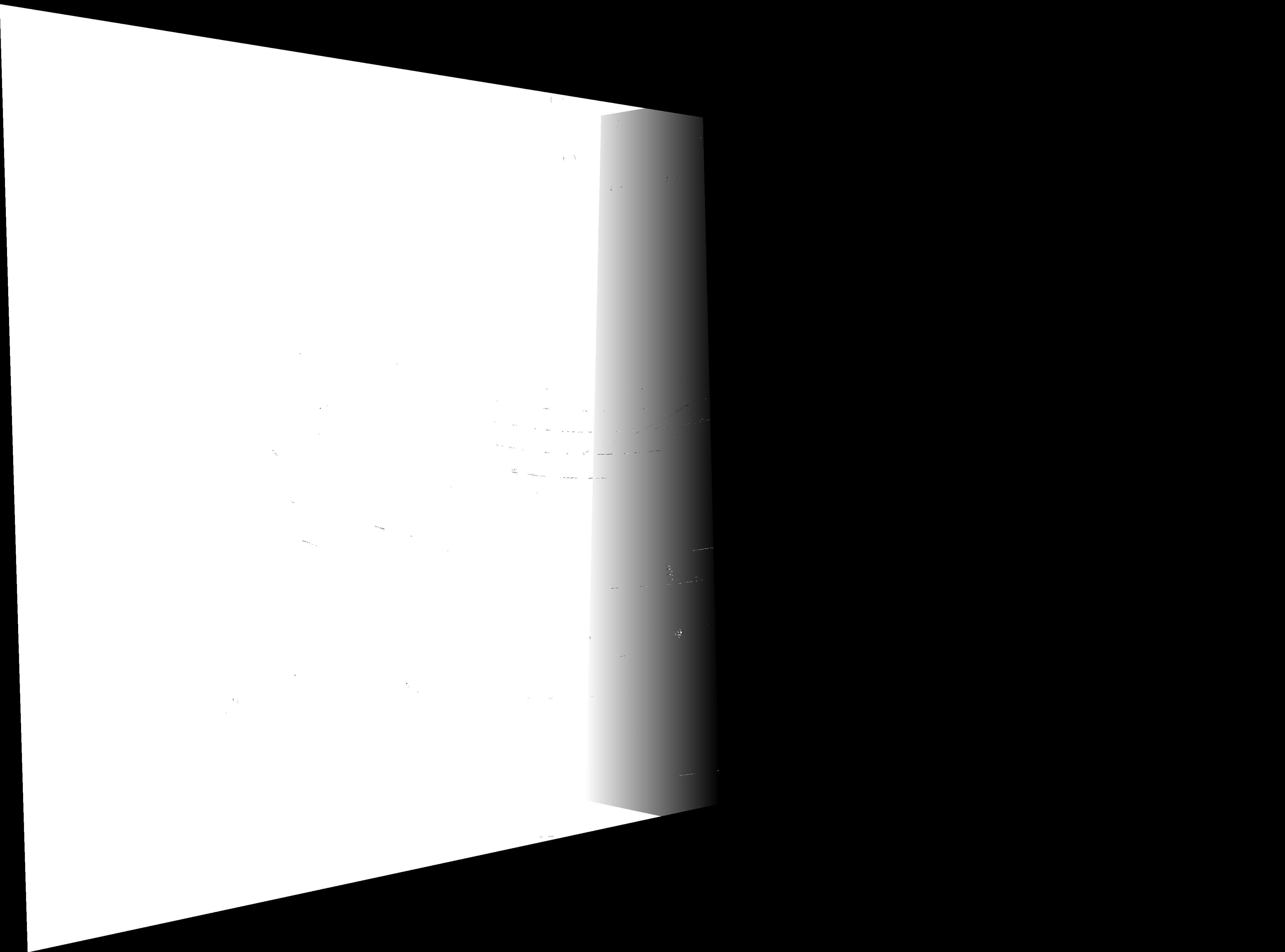
The left mask (feathered).
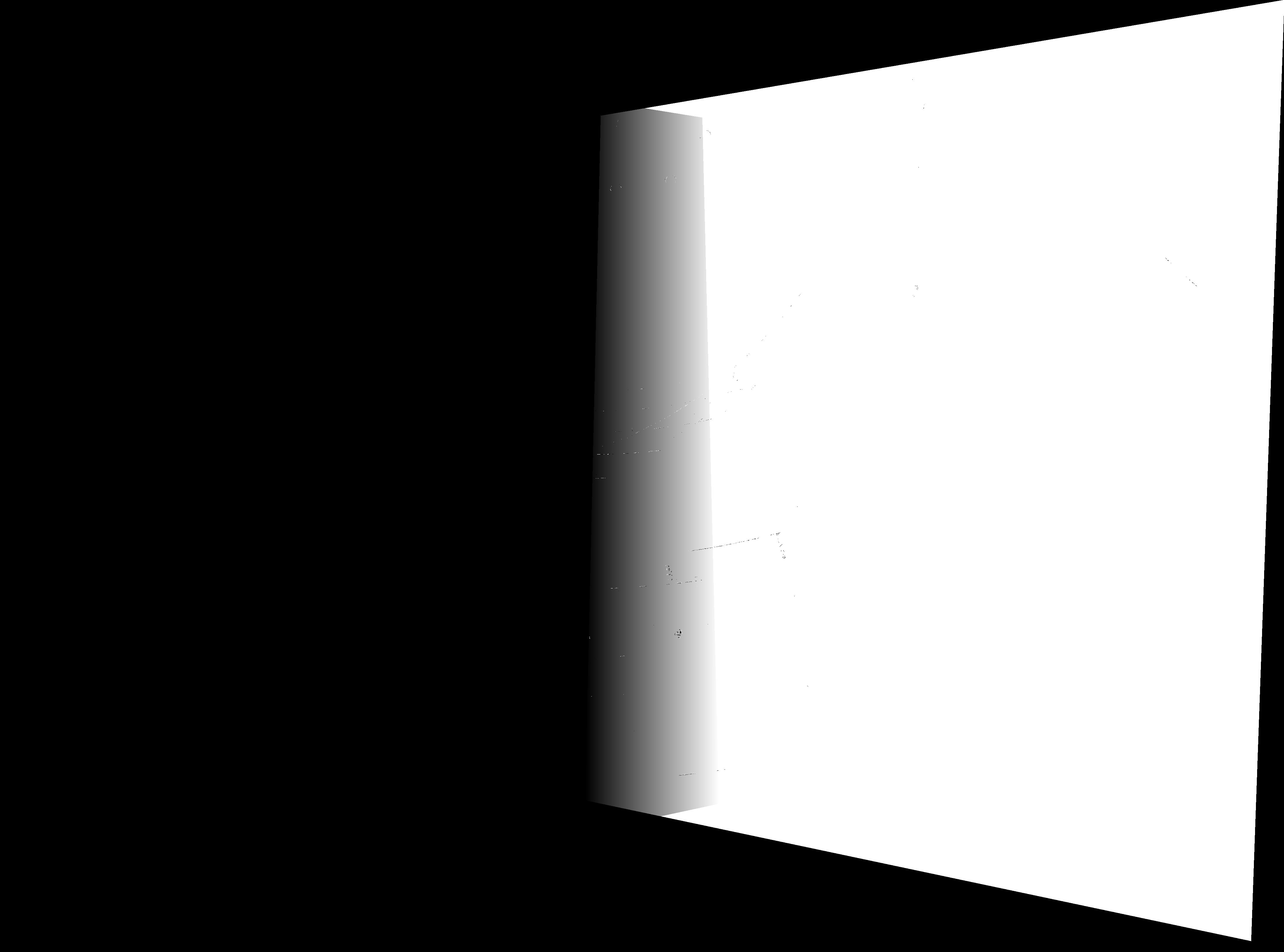
The right mask (feathered).
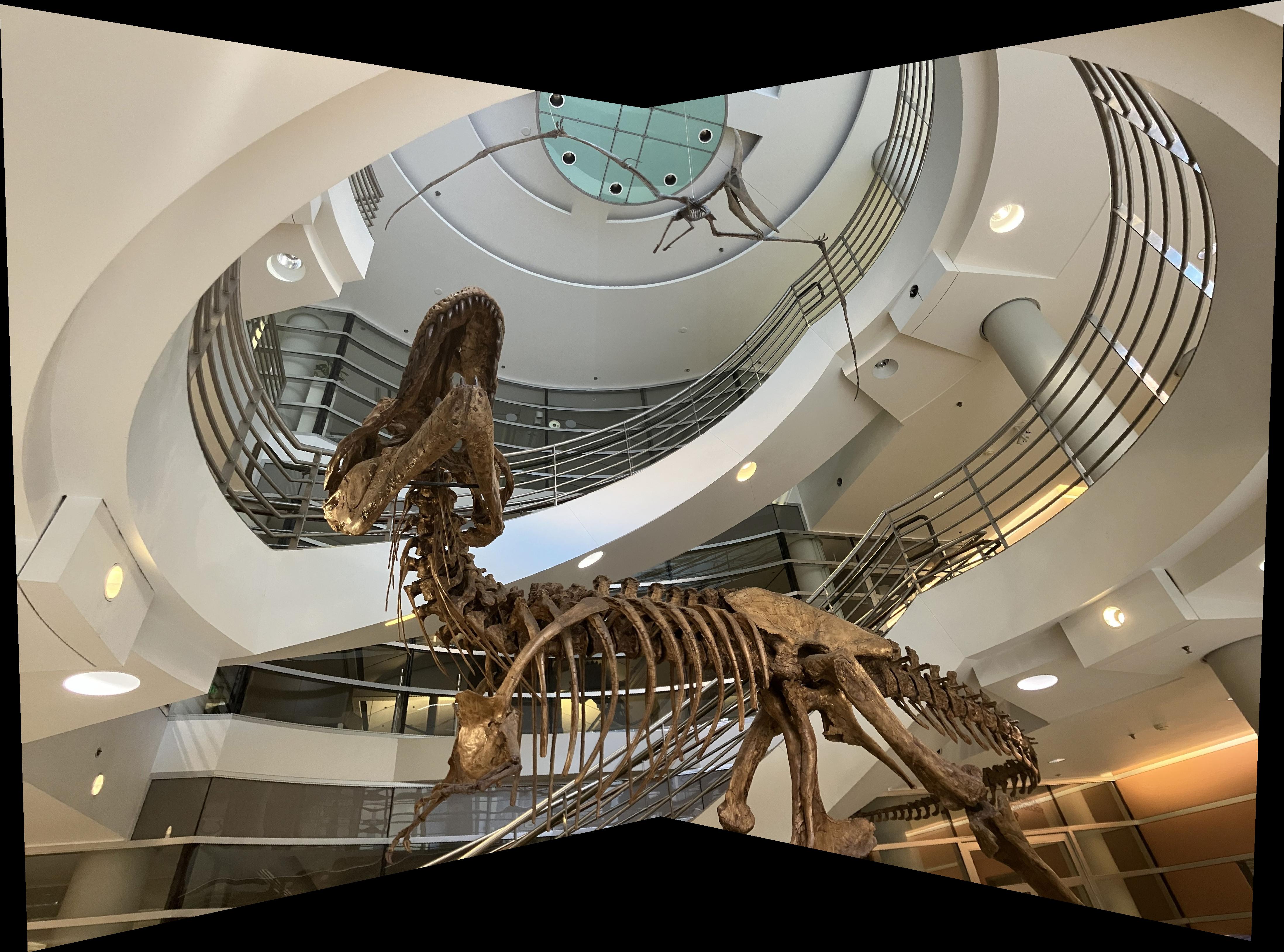
The final mosaic (feathered).
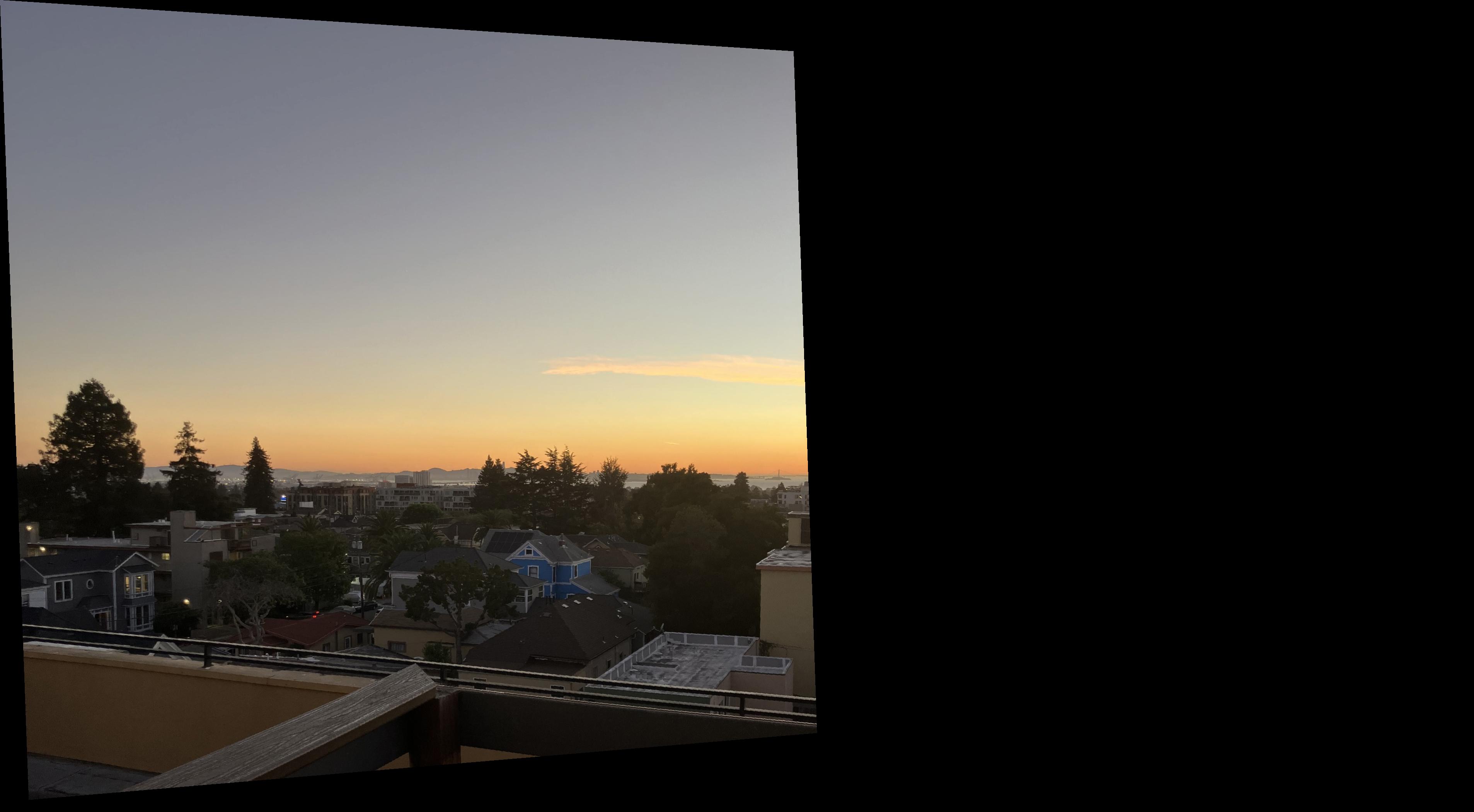
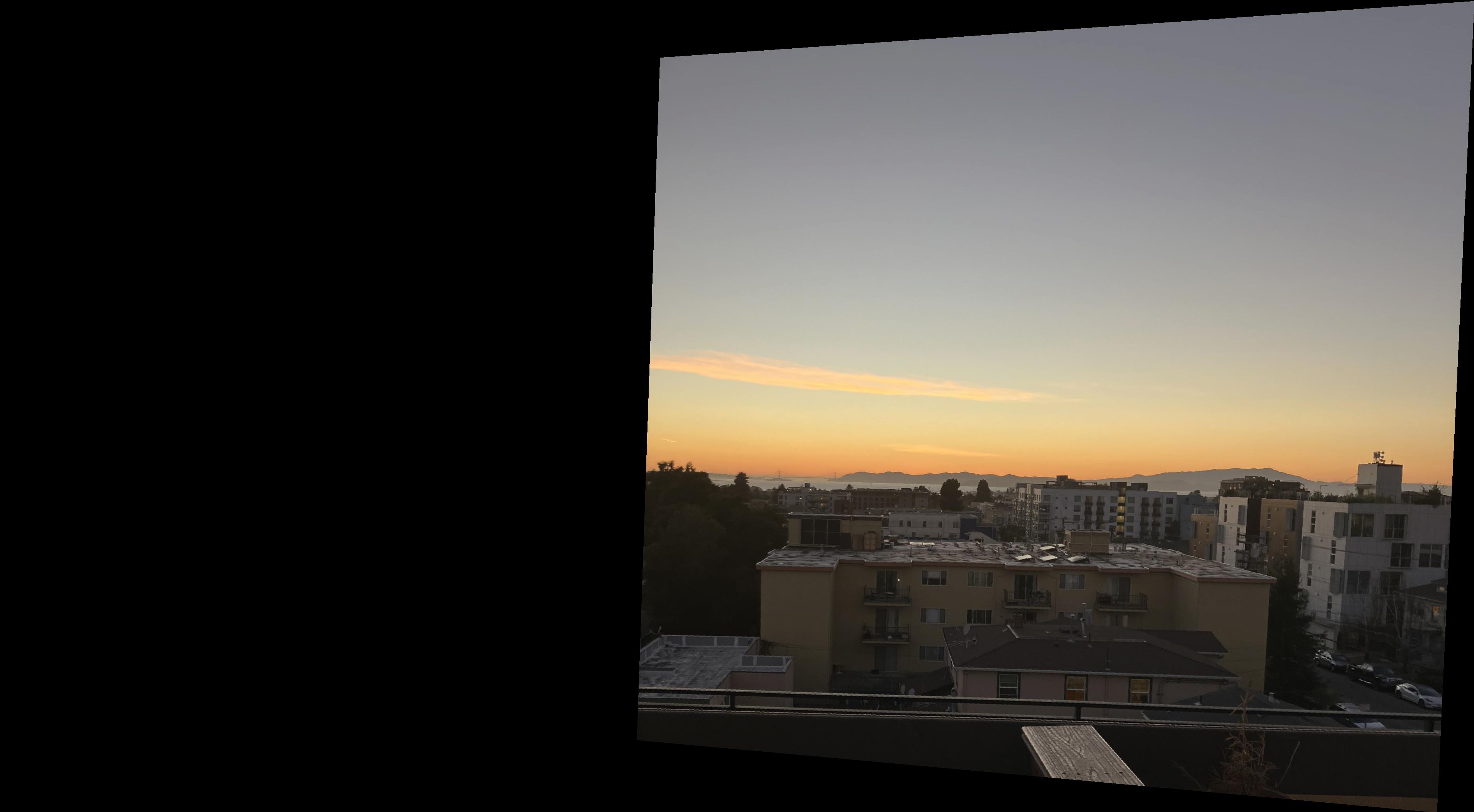
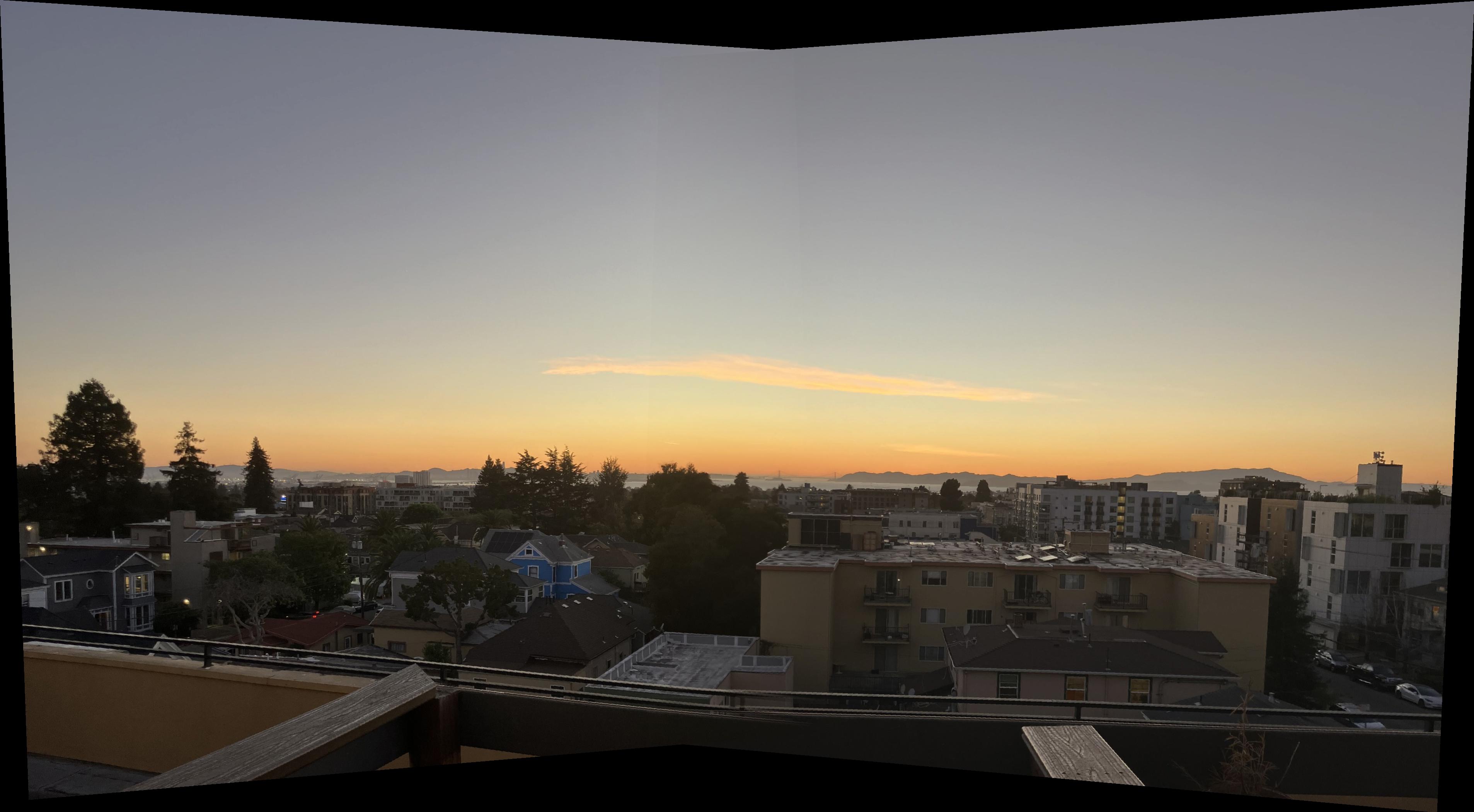
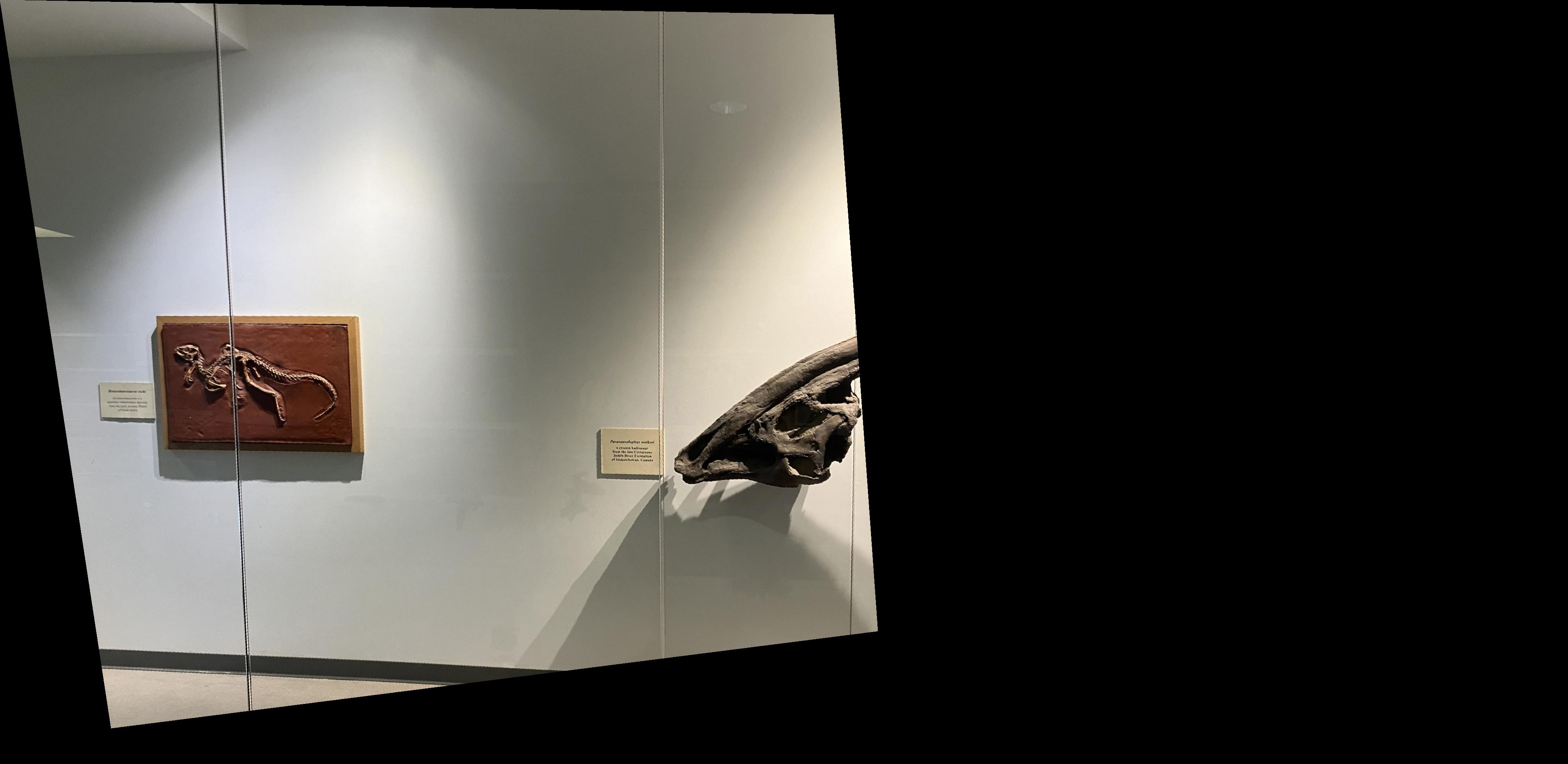
I used the same technique to blend the following images together.
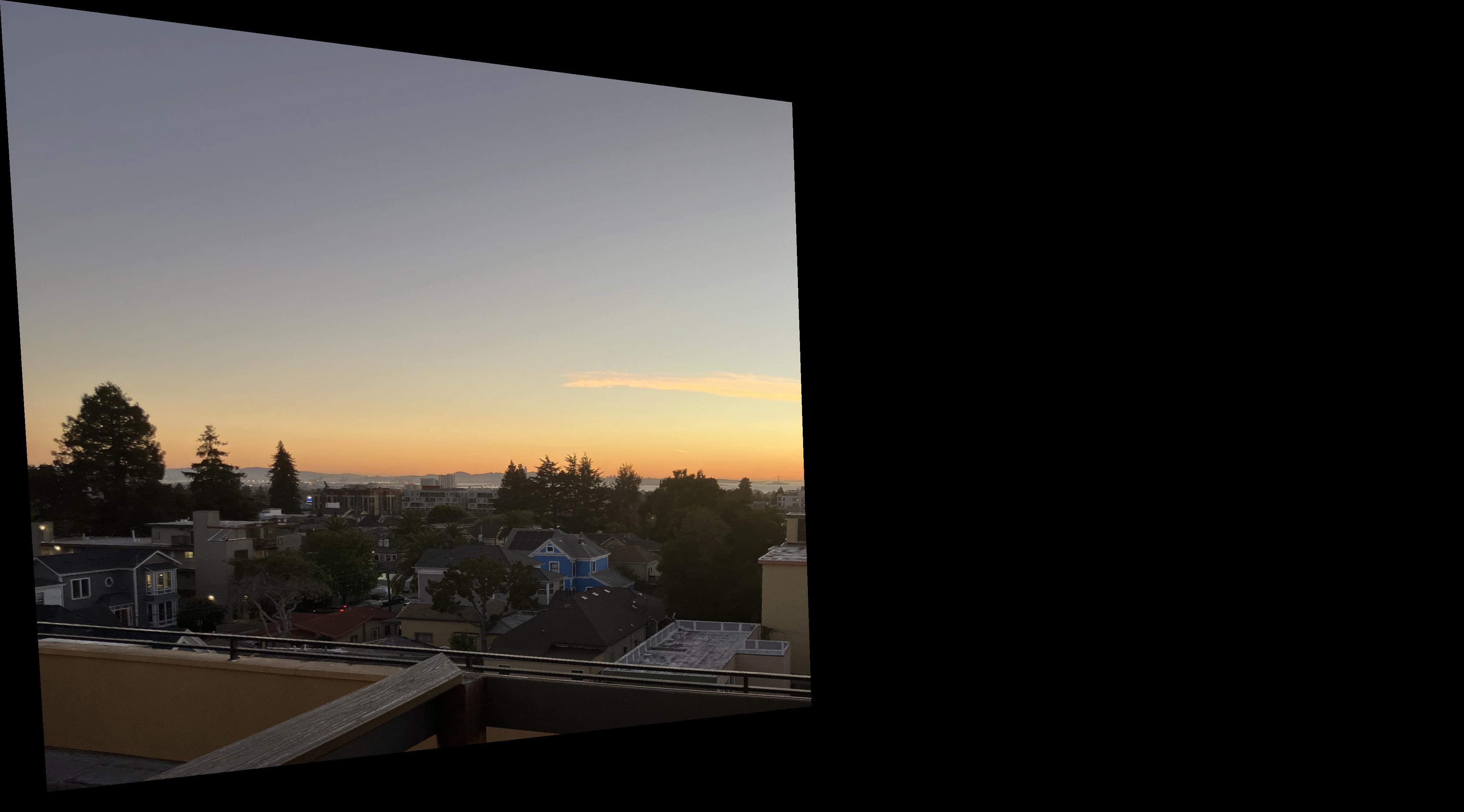
The left image.
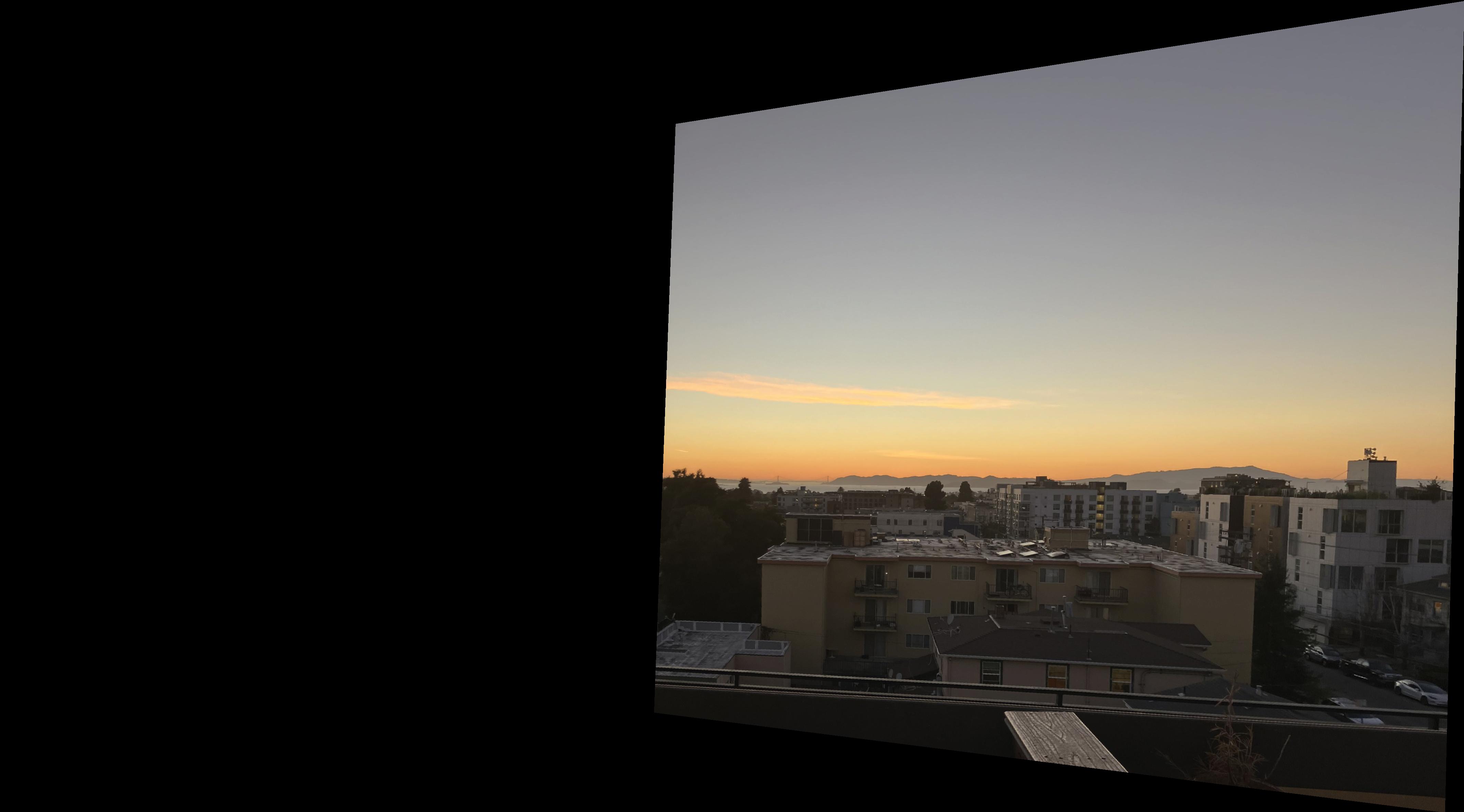
The right image.
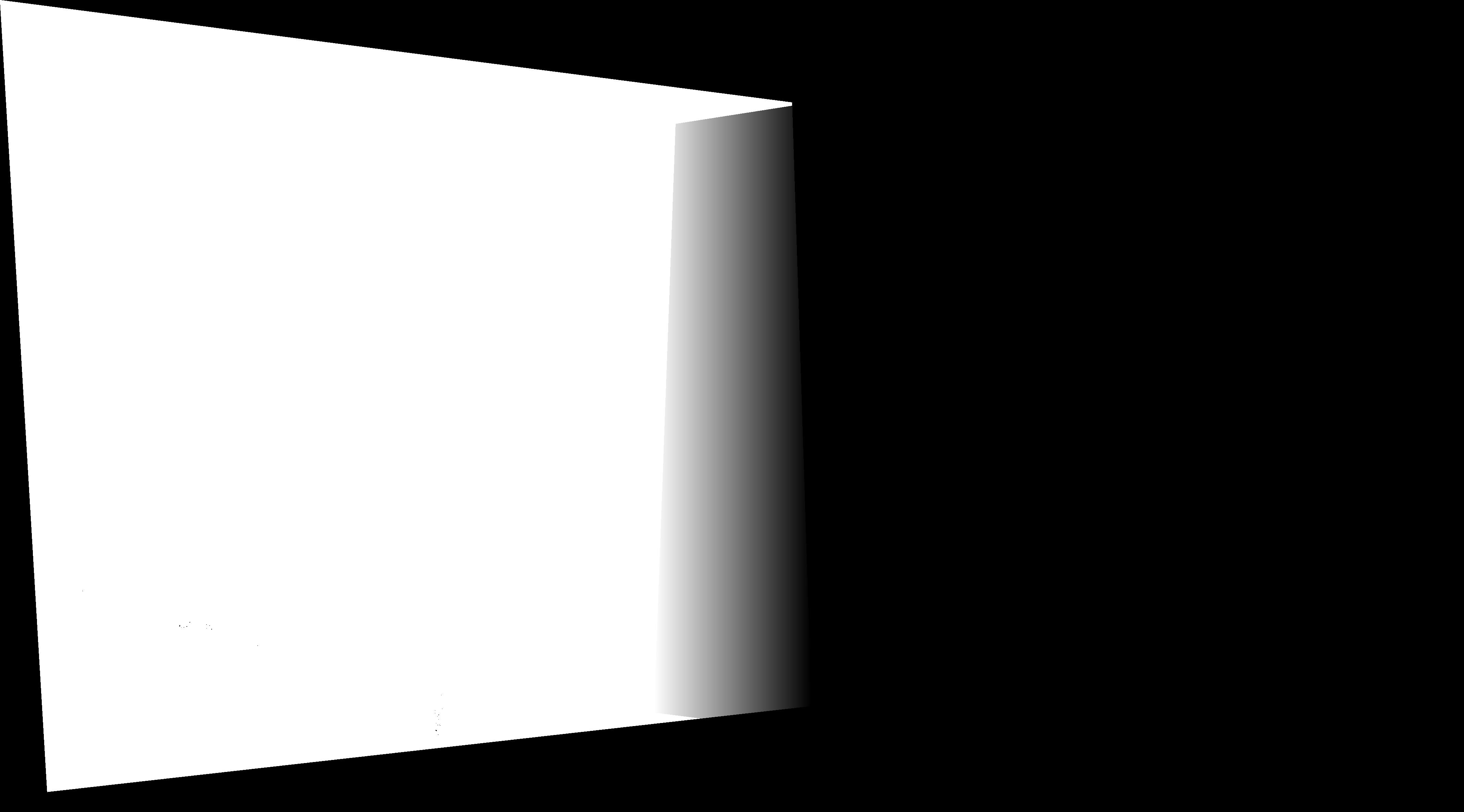
The left mask.
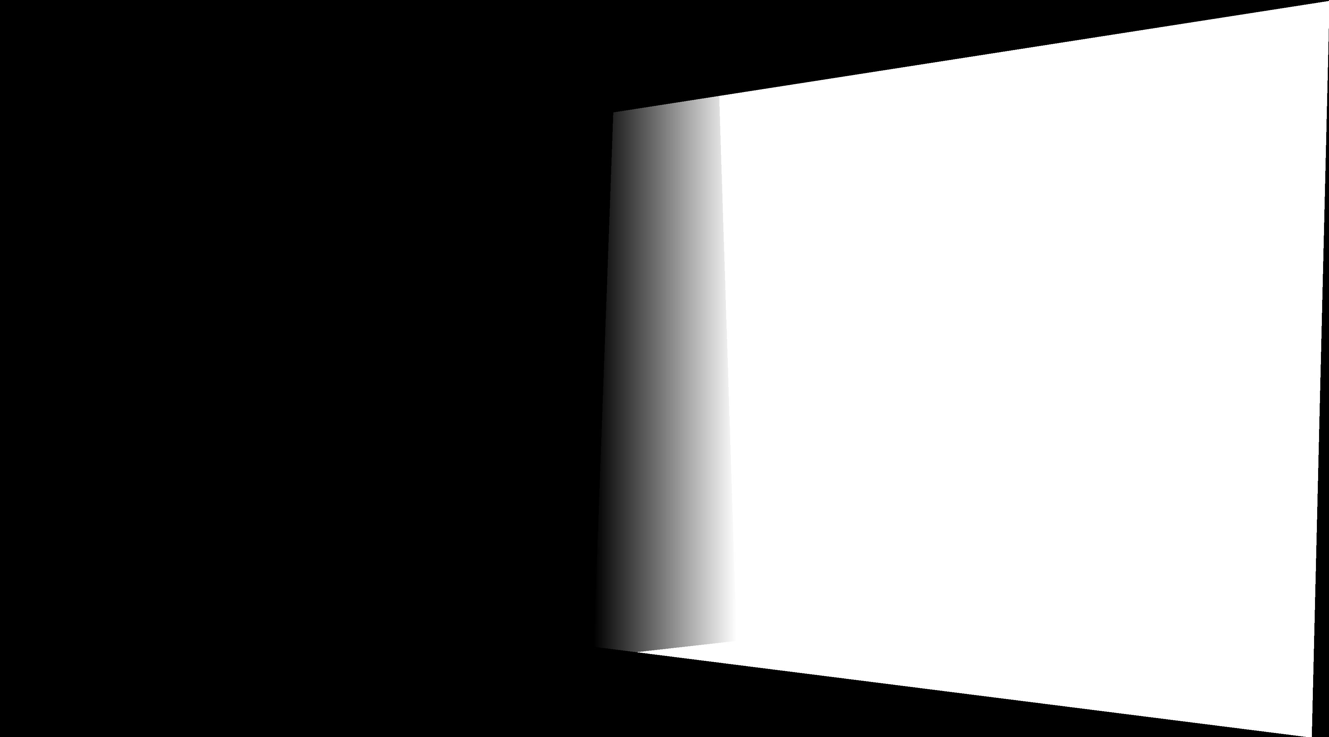
The right mask.
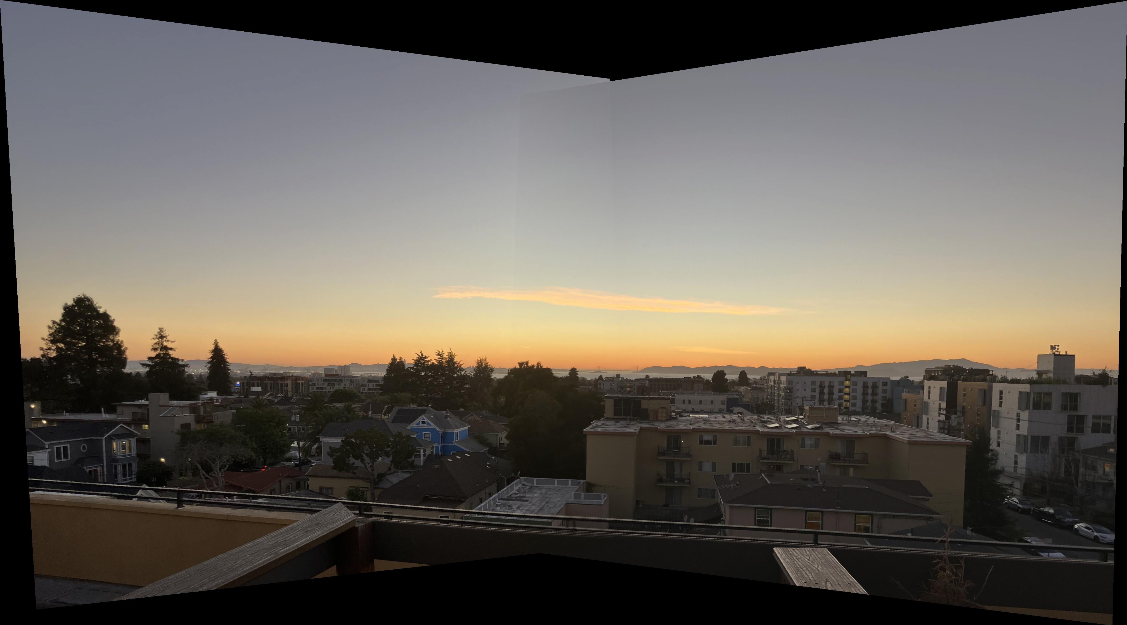
The final mosaic.
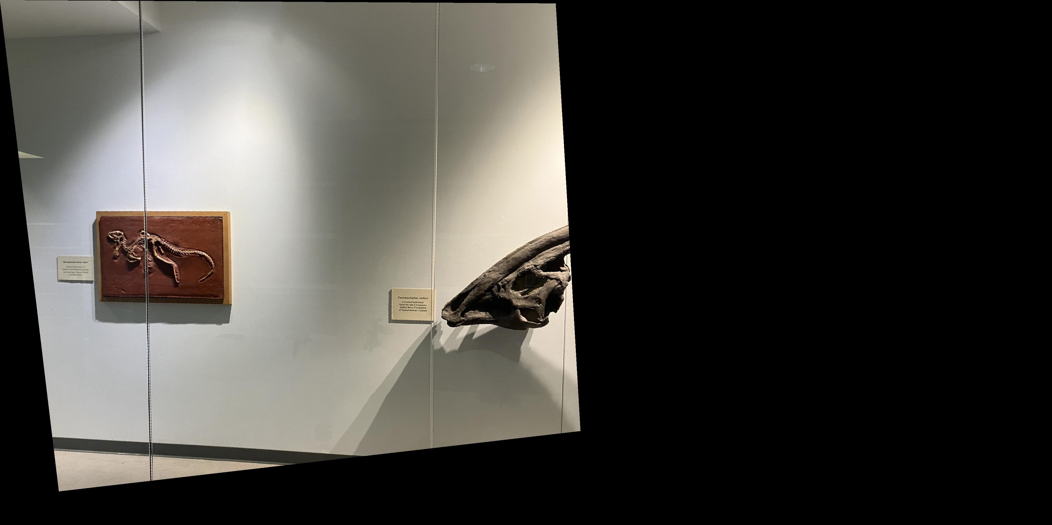
The left image.
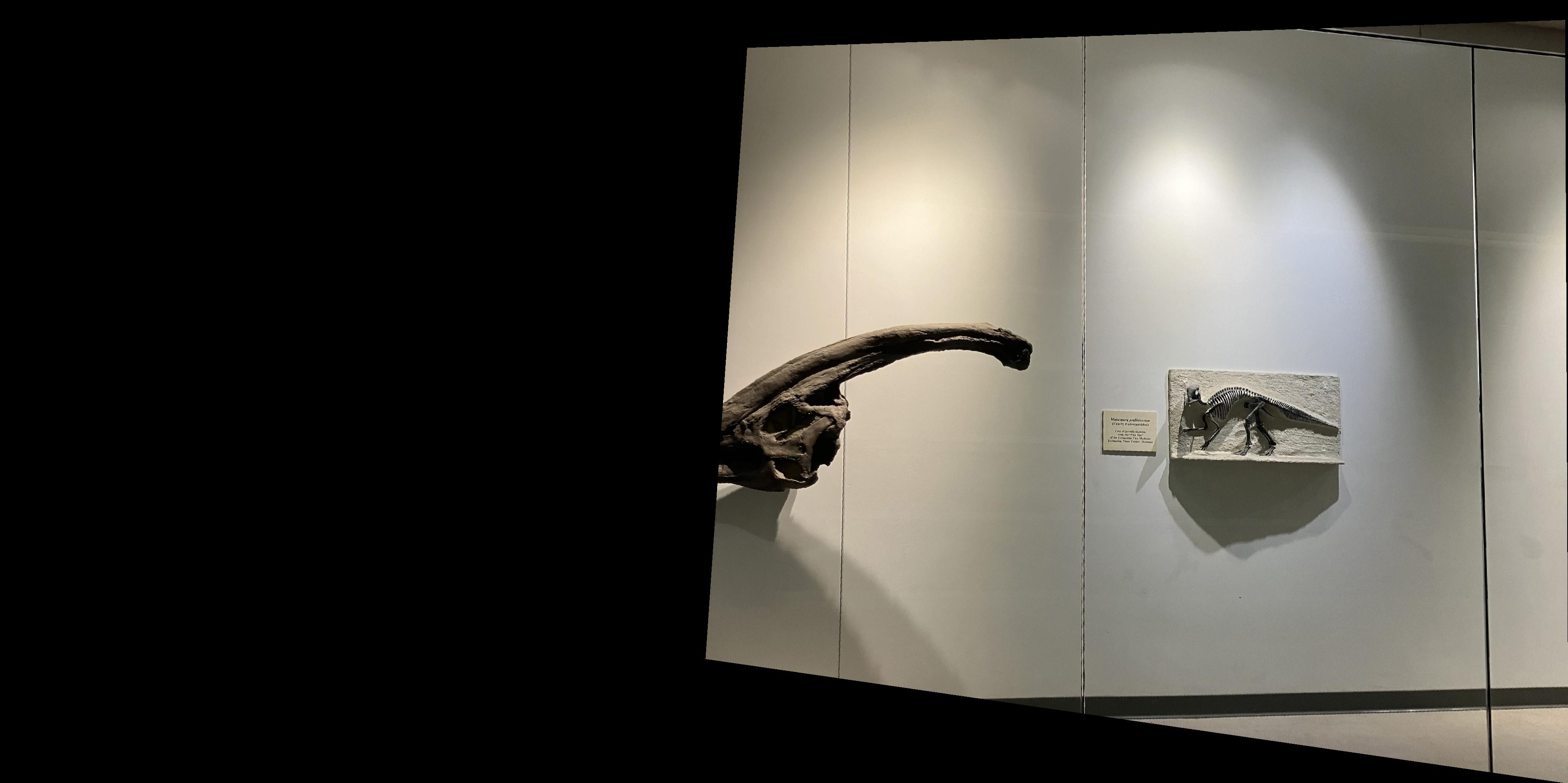
The right image.
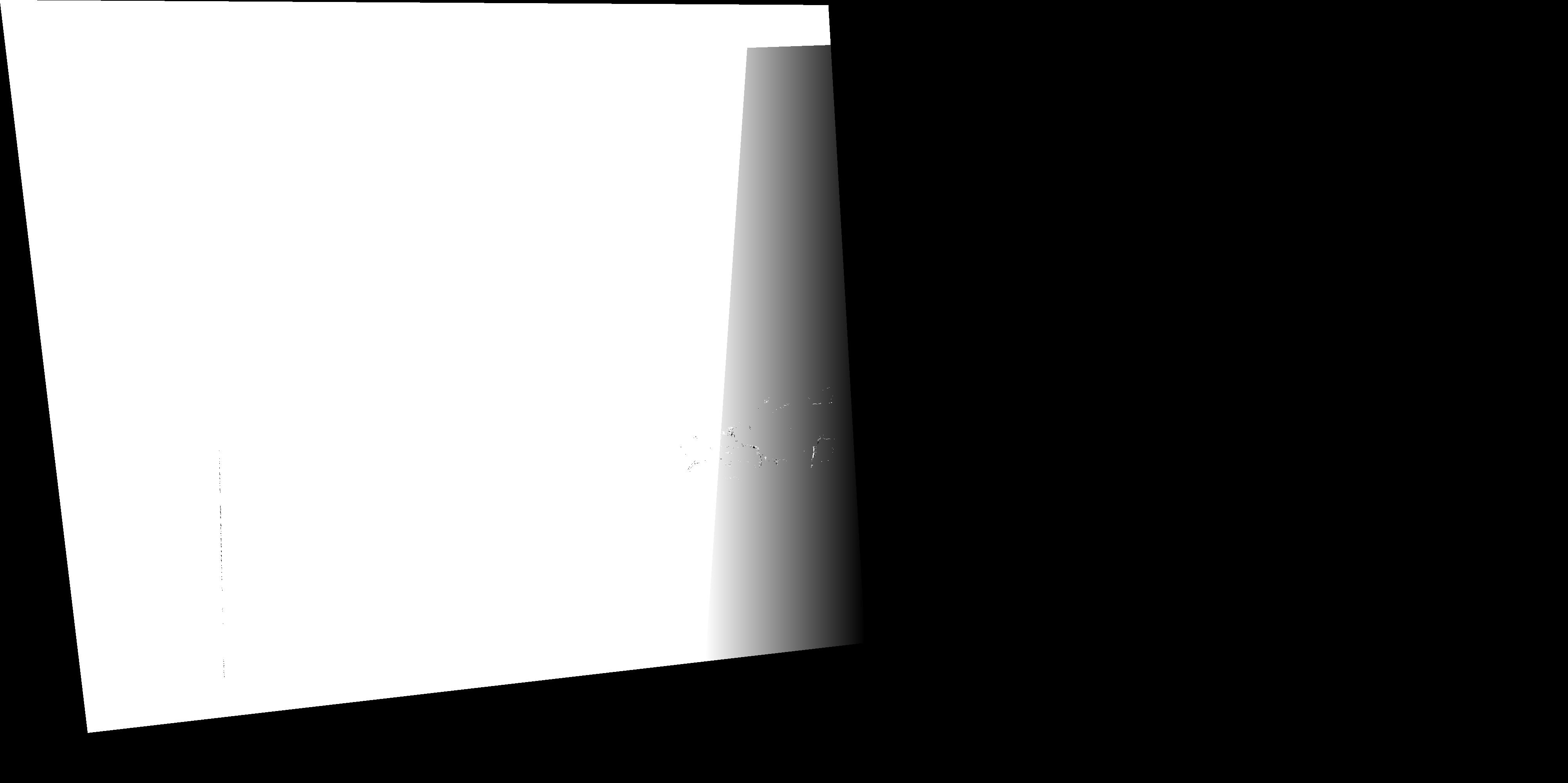
The left mask.
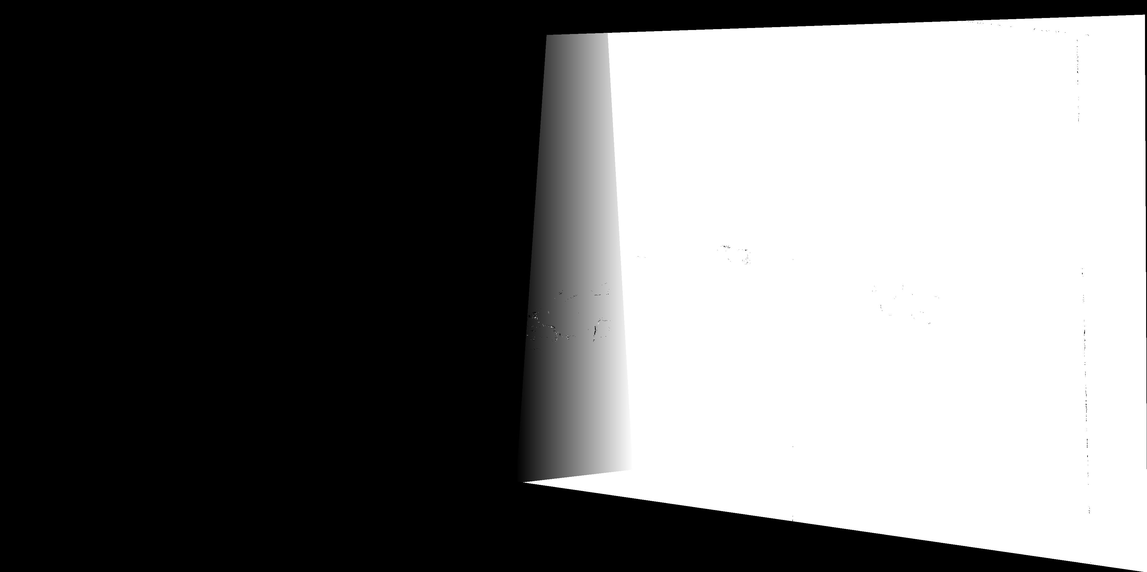
The right mask.
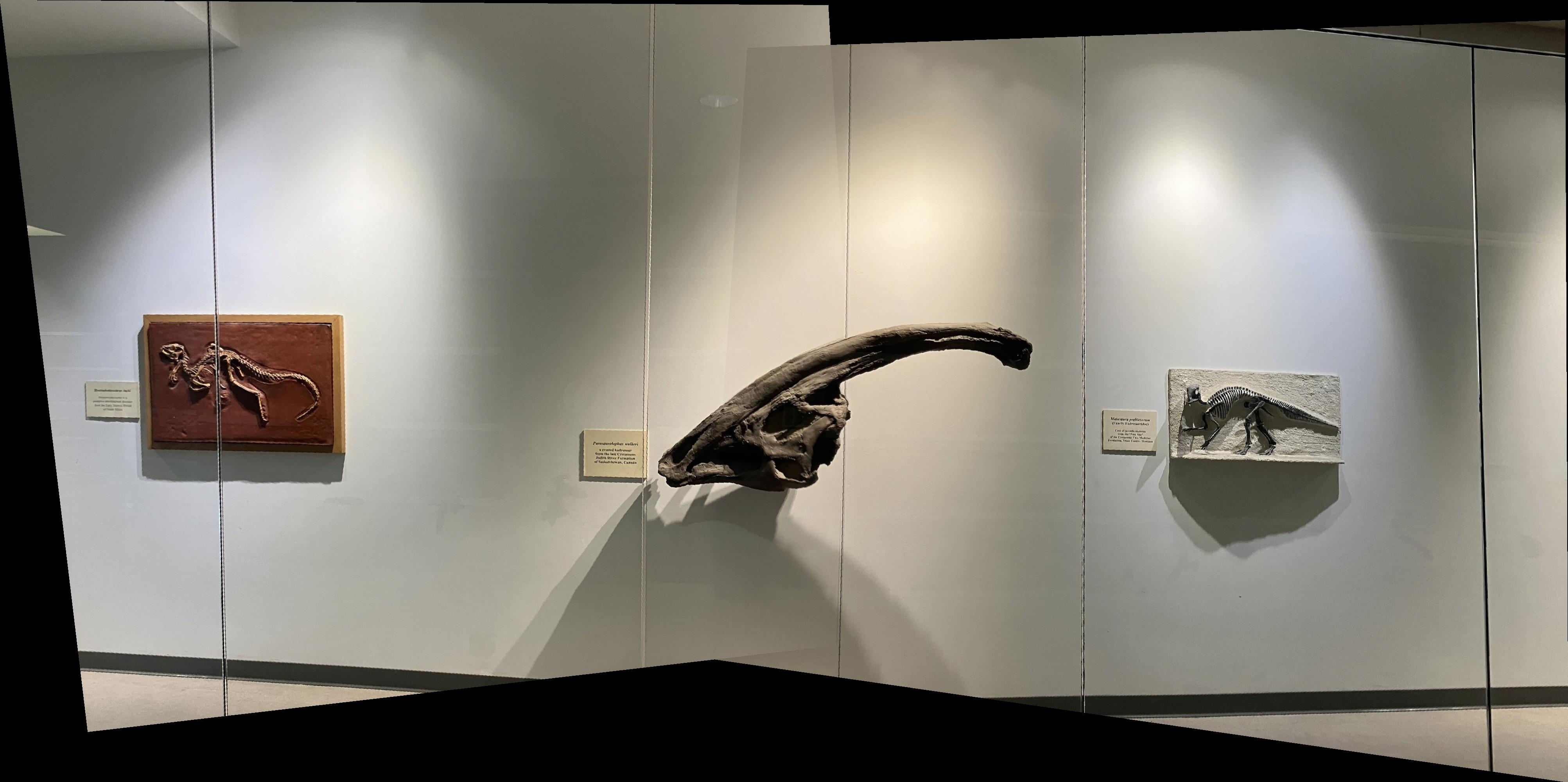
The final mosaic.
