Overview
My goal for this project was to create interesting visual effects by manipulating image frequencies. This involved applying my knowledge of difference operators, low-pass filters, high-pass filters, and more to implement functions such as image sharpening, image hybridization, and image blending. My most important takeaway from the project was a better understanding of the math and logic behind various photo editing tools— actually implementing the methods myself helped me see photo editing as a logical process instead of a black box.
Section I: Fun with Filters
Part 1.1: Finite Difference Operator
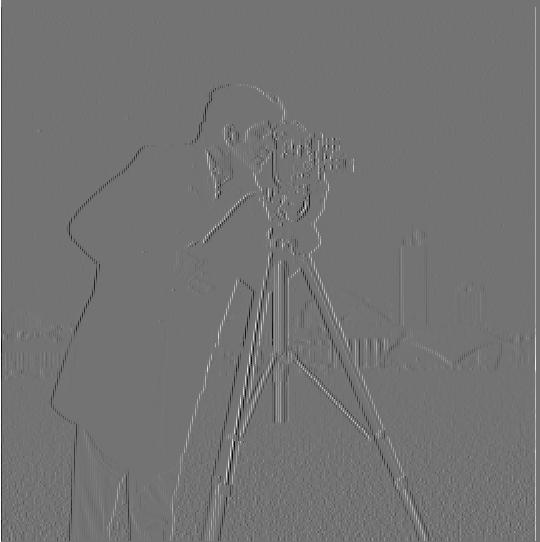
To retain the partial derivatives in x and y of the image, I convolved it with the finite difference operators Dx and Dy, which were simply created with arrays. Next, to obtain the gradient magnitude, I calculated the square root of the sum of the squares of the partial derivatives.


I then binarized the gradient magnitude by iterating through each pixel—if its value was less than some threshold, I set it to 0. If it was greater, I set it to 1. After some trial and error, I decided that a threshold of 0.2 produced the cleanest edge image, as it results in a relatively clear outline while minimizing noise.
cameraman.jpg
Dx
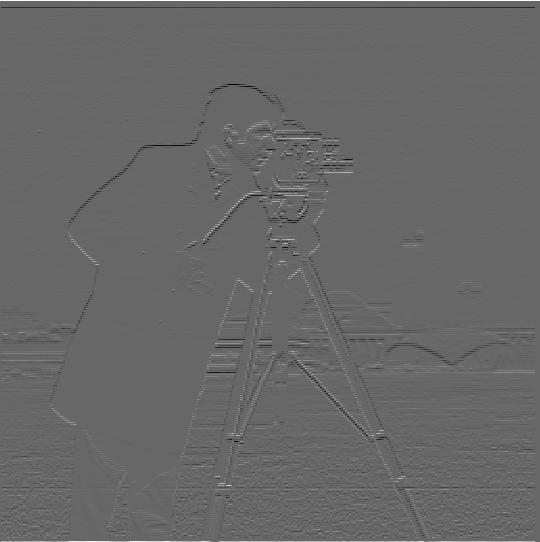
Dy
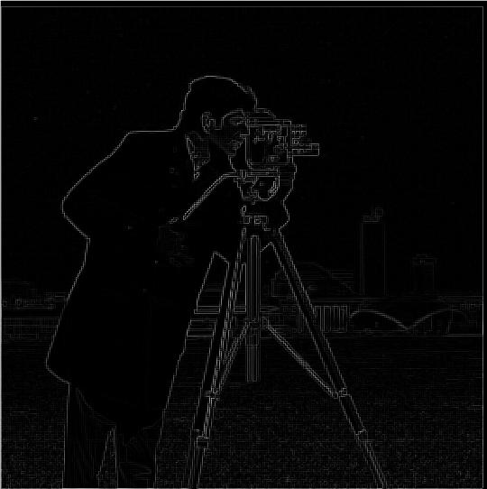
Gradient magnitude
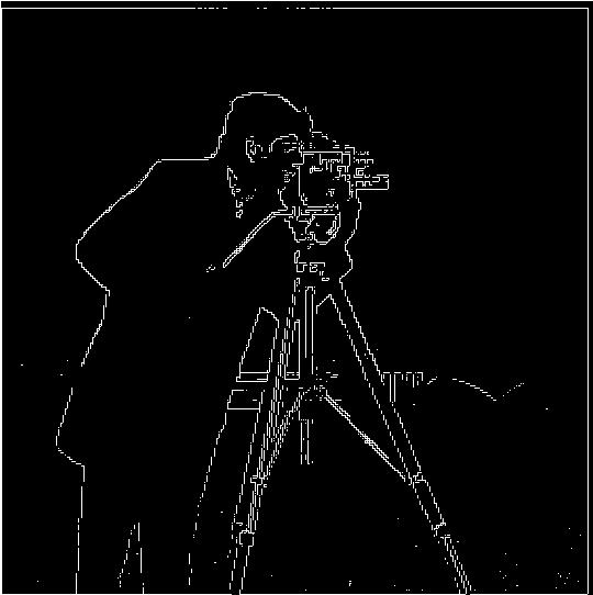
Binarized (threshold = 0.2)
Part 1.2: Derivative of Gaussian Filter
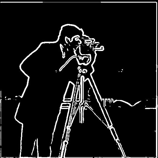
To reduce the amount of background noise in the edge image, I convolved the image with a Gaussian filter before repeating the steps from Part 1.1. The blurred image yielded an edge image with a thicker, smoother outline and less stray pixels.
cameraman.jpg

Dx
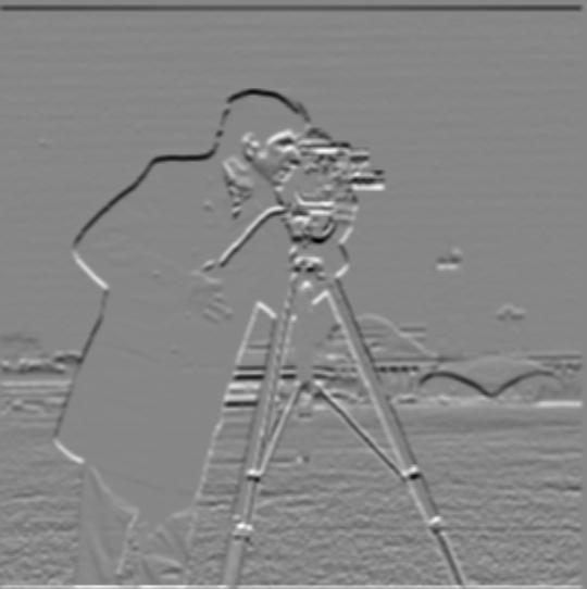
Dy
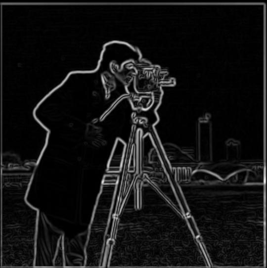
Gradient magnitude

Binarized (threshold = 0.3)
As a sanity check, I also convovled the Gaussian filter directly with Dx and Dy to achieve the same results with less convolutions.
cameraman.jpg
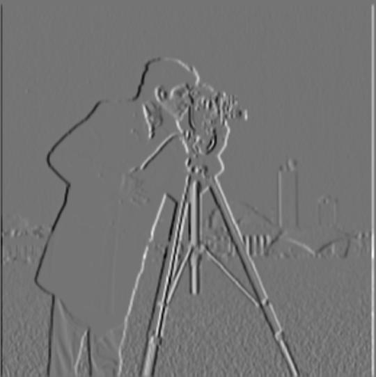
Dx
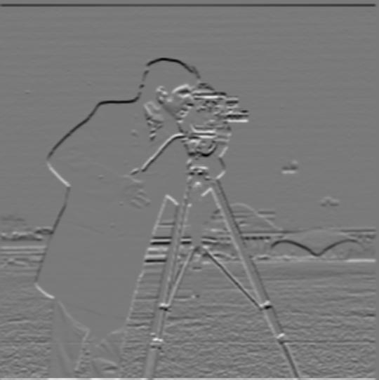
Dy
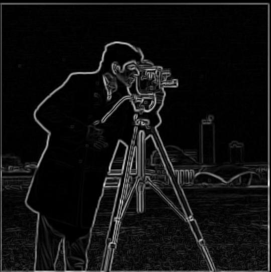
Gradient magnitude
Binarized (threshold = 0.3)
Section II: Fun with Frequencies
Part 2.1: Image "Sharpening"
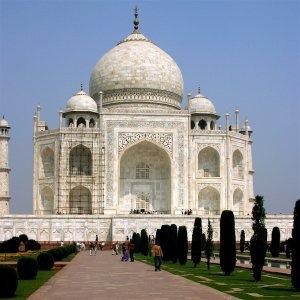
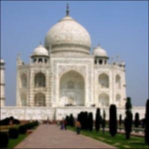
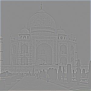
Next, I implemented the unsharp masking technique. To isolate the low frequencies of an image, I convolved the image with a Gaussian filter. To isolate the high frequencies, I subtracted the blurred image from the original image. Finally, I combined the original image with the high frequencies multiplied by an alpha, making the high frequencies more prominent; this "sharpens" an image. I combined the steps into a single convolution called the unsharp filter.
taj.jpg
Original (a = 0)
Low frequency
High frequency
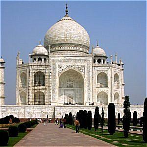
a = 1
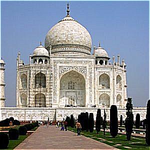
a = 2
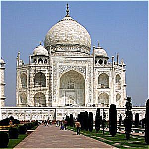
a = 3
dog.jpg

Original (a = 0)

Low frequency
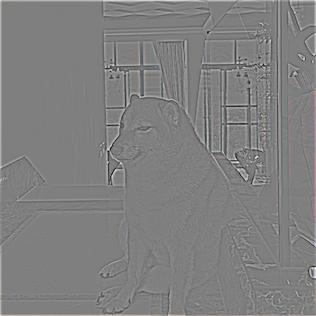
High frequency
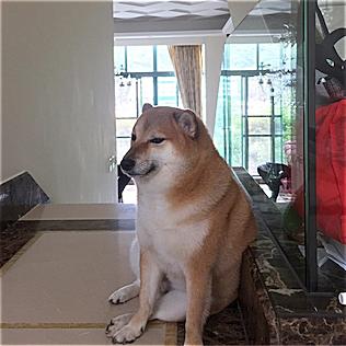
a = 1
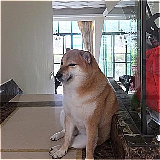
a = 2
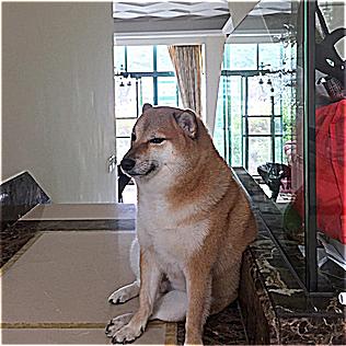
a = 3
moodeng.jpg
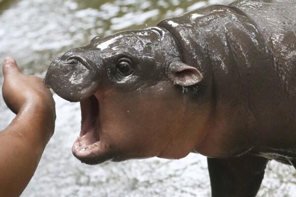
Original (a = 0)

Low frequency
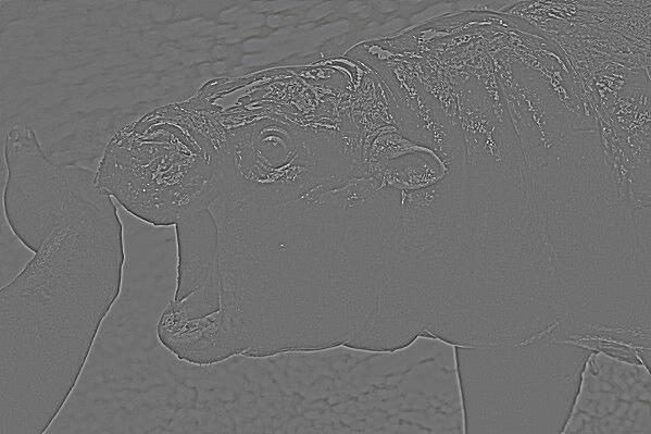
High frequency

a = 1
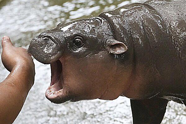
a = 2

a = 3
I also experimented with blurring images beforehand. Although sharpening captured most of the original details, the result appears grainier than desired.
frog.jpg

Original (a = 0)

Blurred
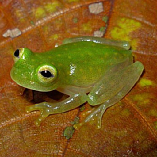
Sharpened (a = 3)
Part 2.2: Hybrid Images
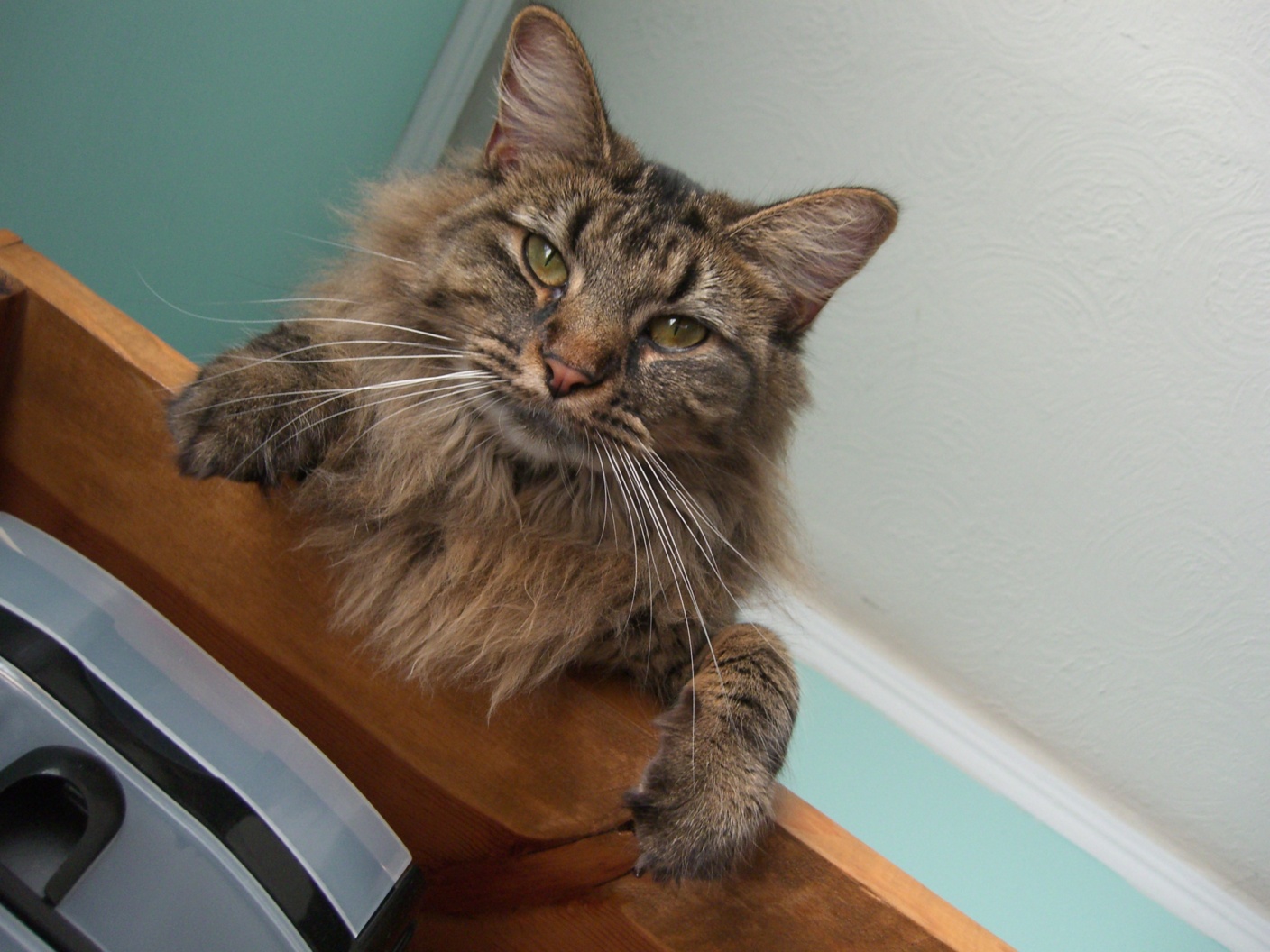
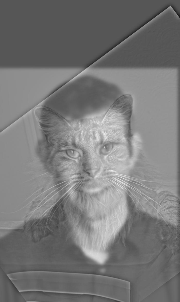
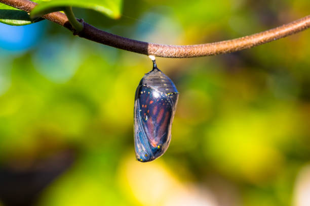
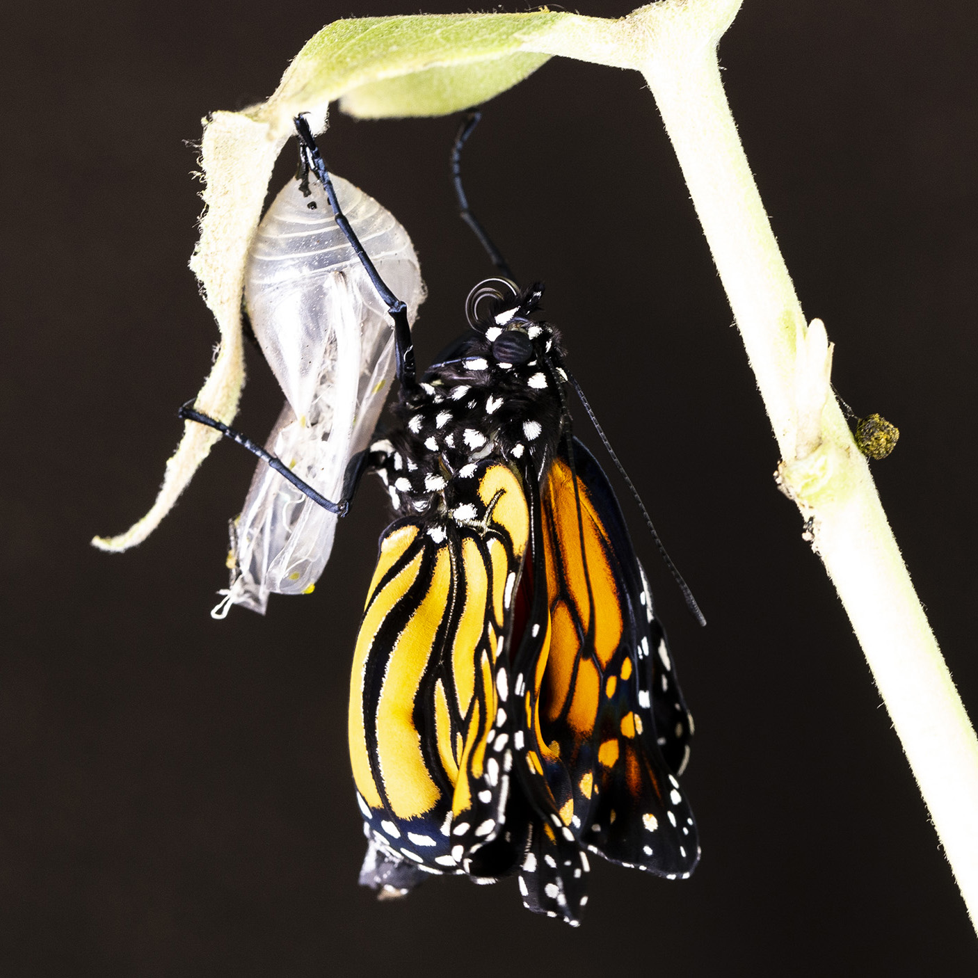
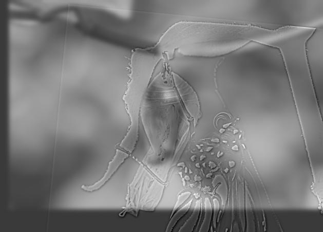
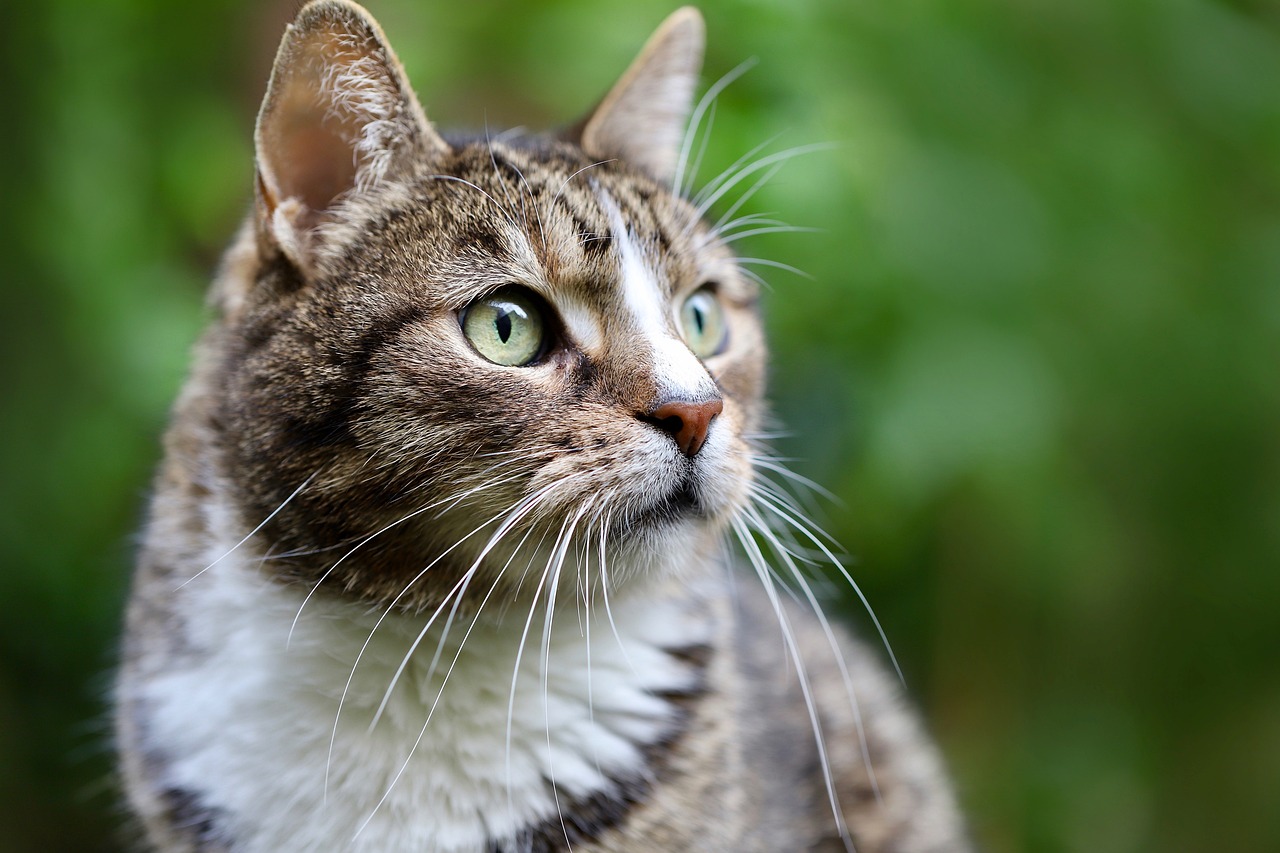
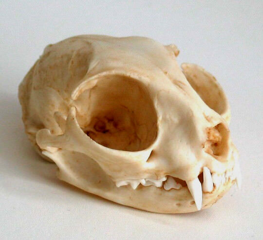
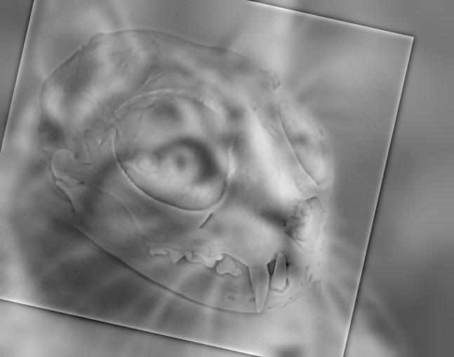
I also implemented image hybridization by blending the high frequencies of one image with the low frequencies of another. Hybrid images are images that are perceived differently based on the viewing distance—the high frequencies are more visible up close, while the low frequencies are more visible at a distance.
Similar to my approach in Part 2.1, I retained the low frequencies of an image by convolving it with a Gaussian filter. I then obtained the high frequencies of another image by subtracting its low frequencies from the original. Taking the average of these two images creates the final result.
DerekPicture.jpg
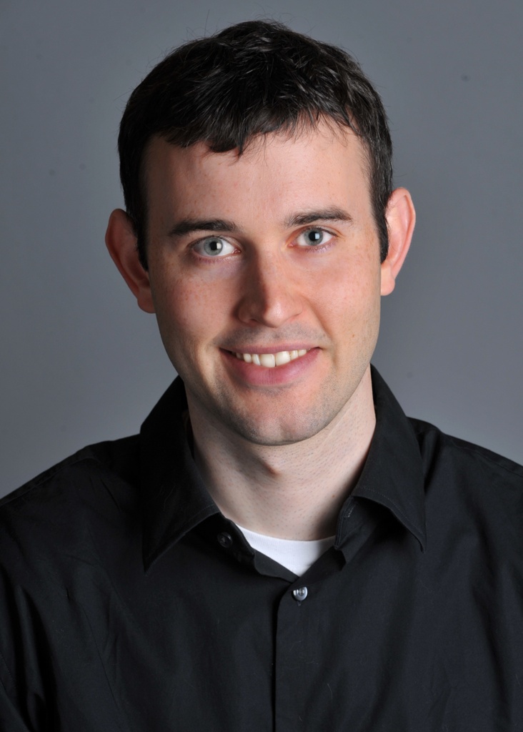
Low frequency
nutmeg.jpg
High frequency
Derek_nutmeg_final.jpg
Hybridized
coccoon.jpg
Low frequency
butterfly.jpg
High frequency
butterfly_coccoon_final.jpg
Hybridized
Favorite Case
cat.jpg
Low frequency
skull.jpg
High frequency
skull_cat_final.jpg
Hybridized
Frequency Analysis

Original
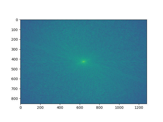
Fourier transform
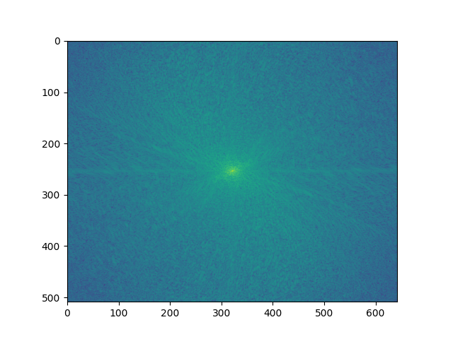
Fourier transform (aligned)

Original
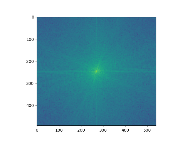
Fourier transform
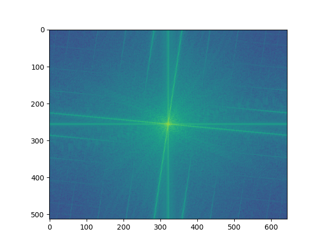
Fourier transform (aligned)

Original
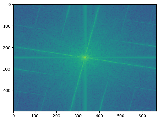
Fourier transform
Failure Case
I had some difficulties blending jinx.jpg with powder.jpg. Jinx's eye is overpowering even at a distance, and it's hard to differentiate between Jinx and Powder's hair up close. This may be due to the stylized nature of the images.
powder.jpg
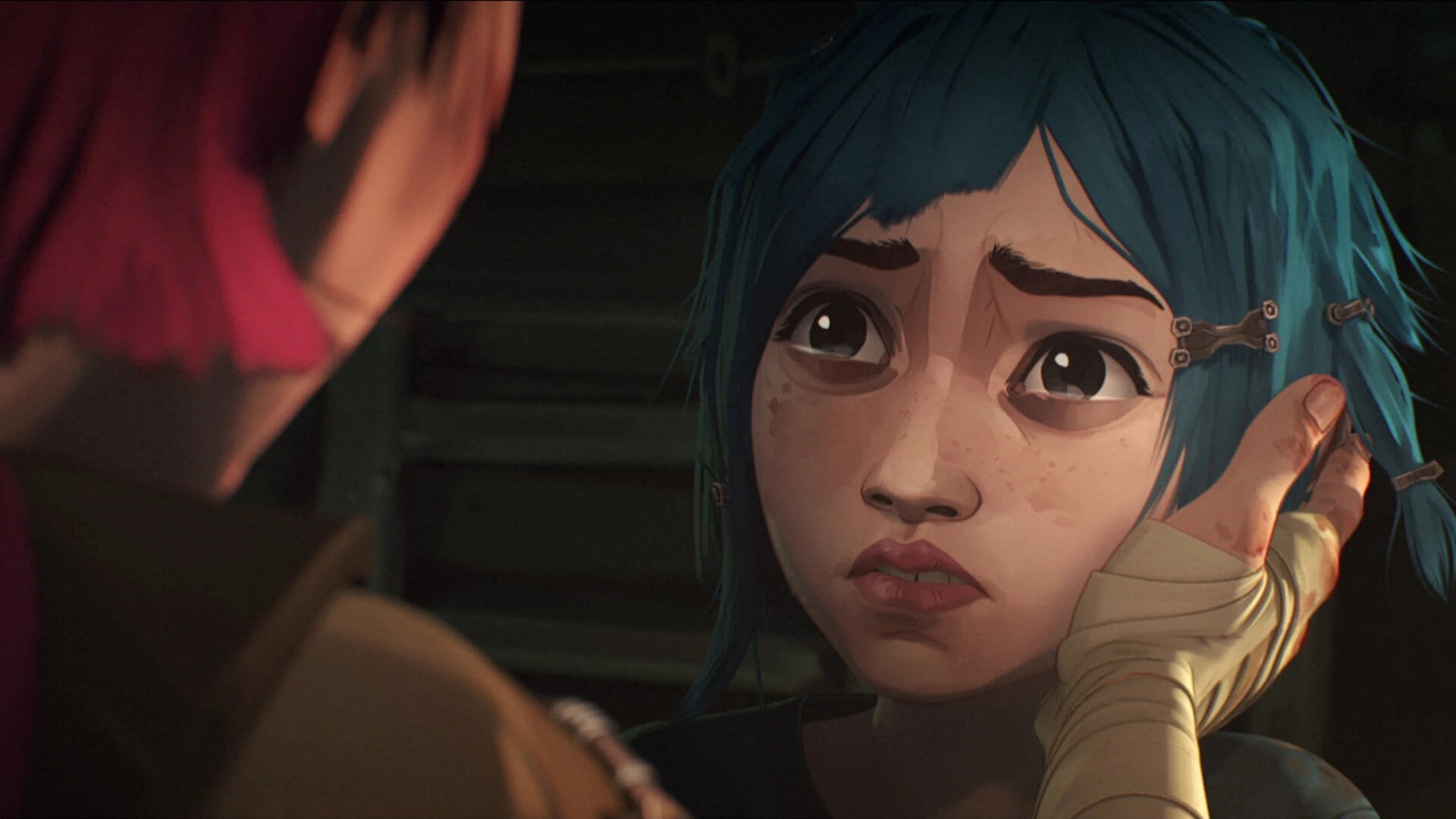
Low frequency
jinx.jpg
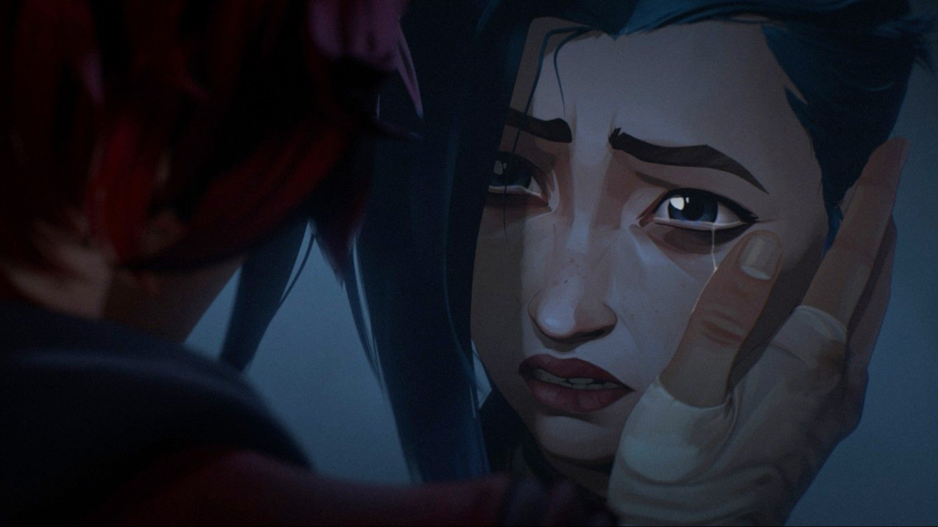
High frequency
jinx_powder_final.jpg
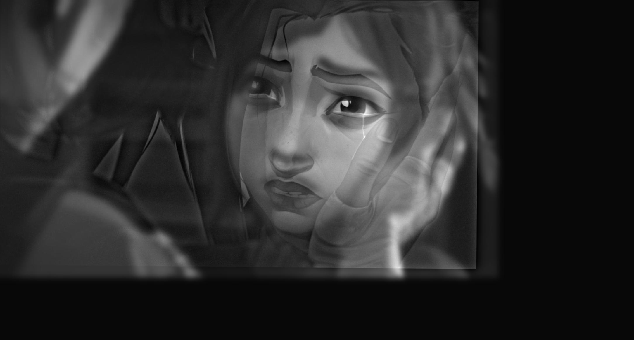
Hybridized
Part 2.3: Gaussian and Laplacian Stacks
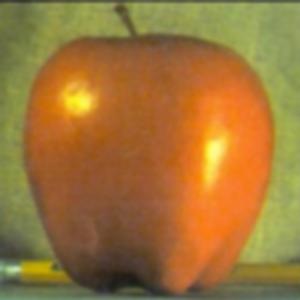
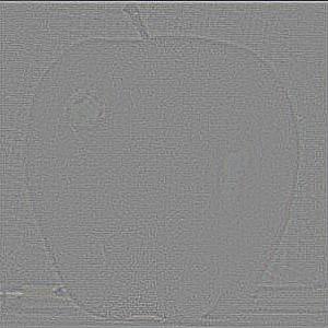
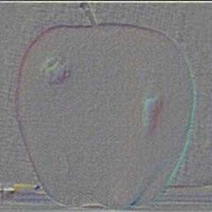
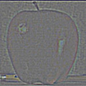
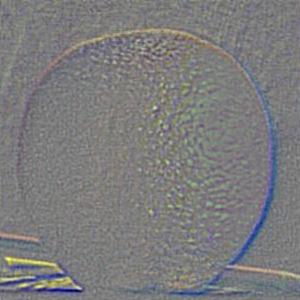
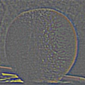
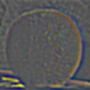
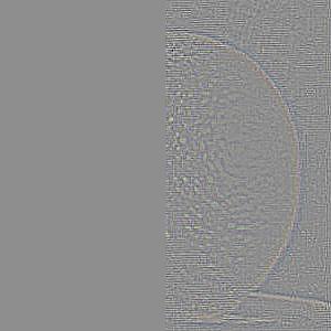
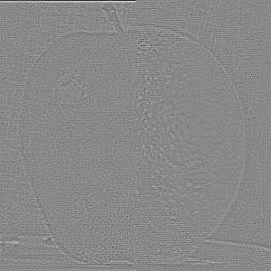
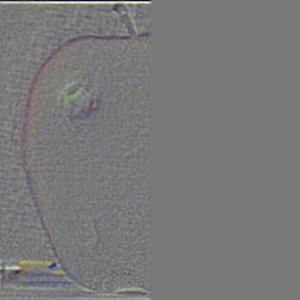
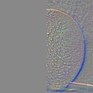
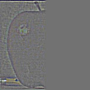
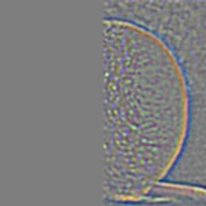
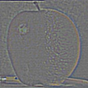
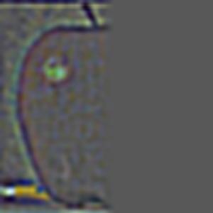
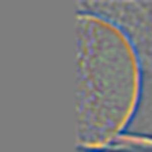
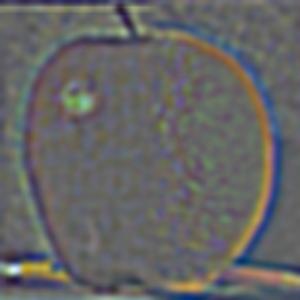
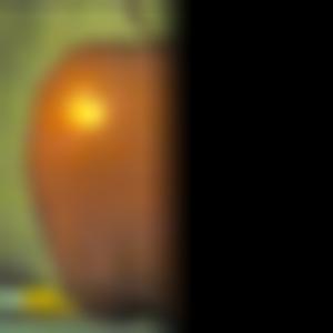
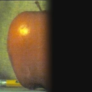
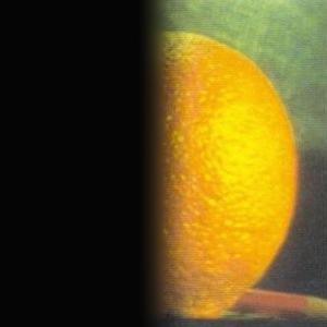
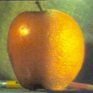
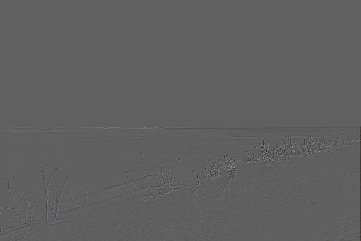
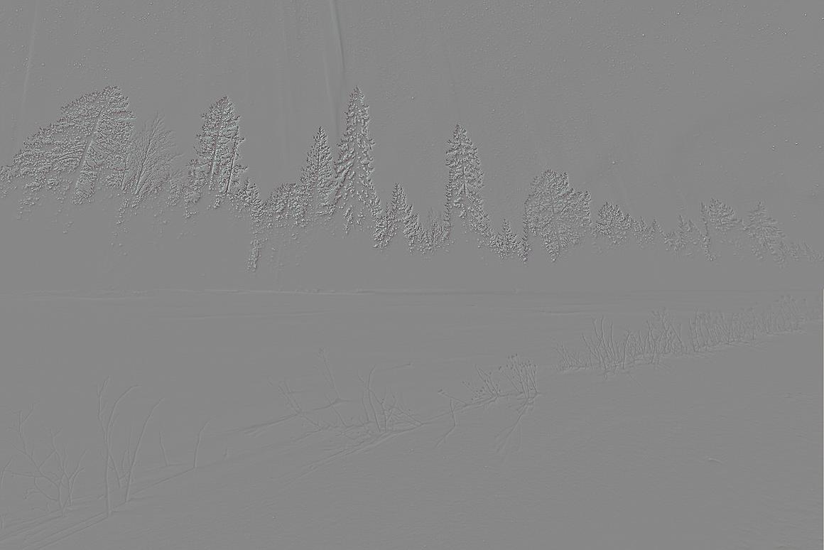
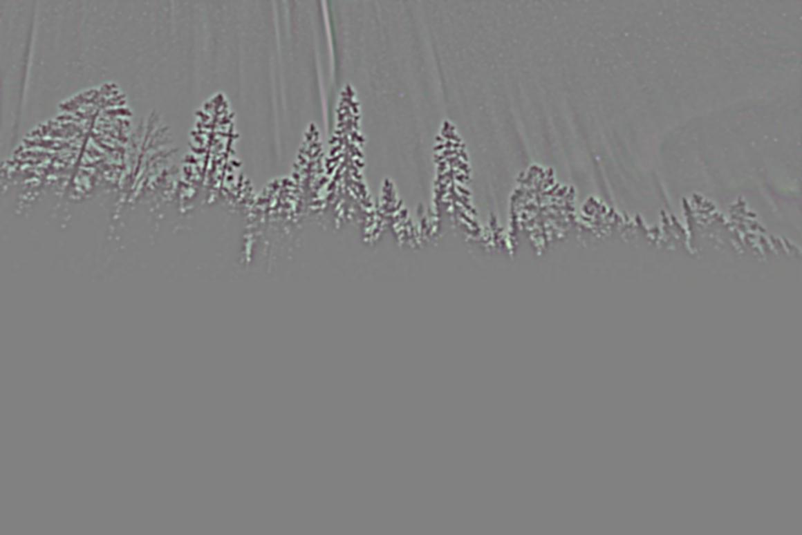
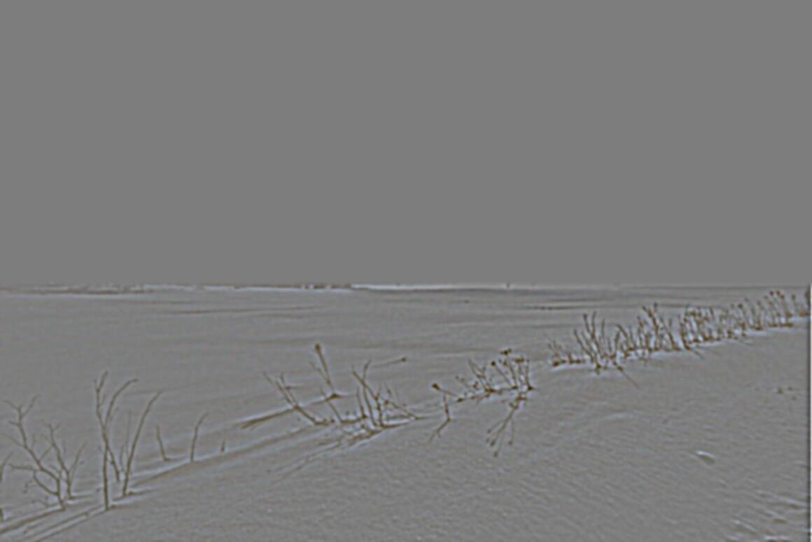
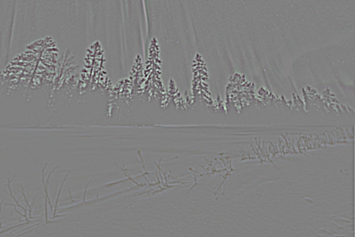
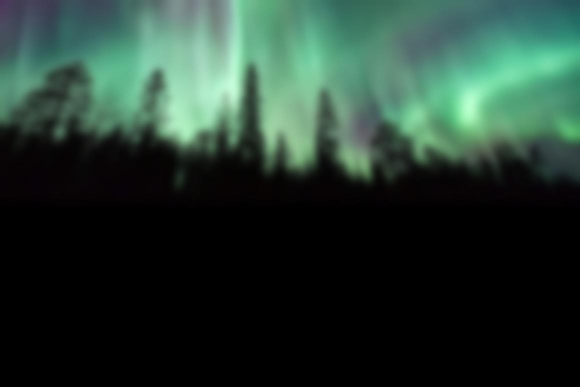
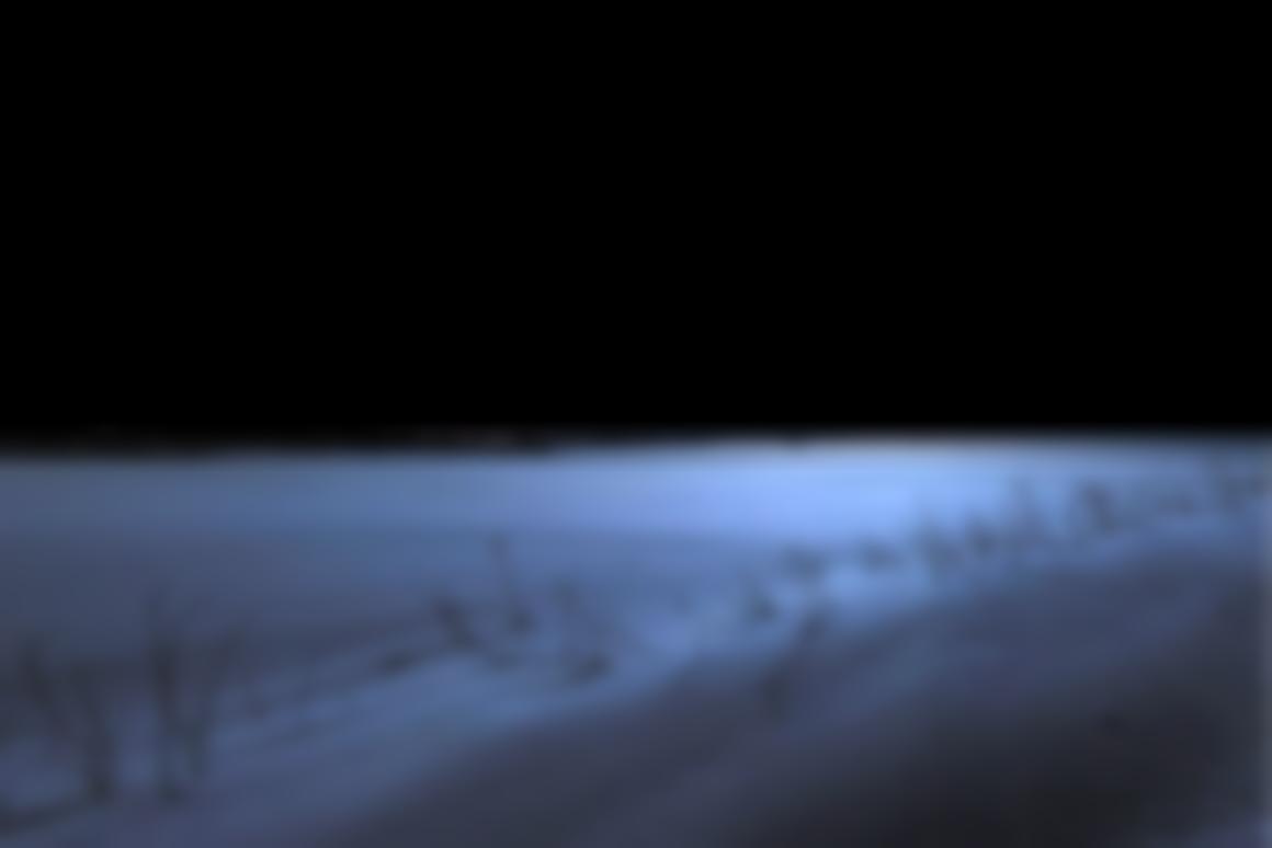
In preparation for multiresolution blending, I implemented Gaussian and Laplacian stacks. To create the Gaussian stack, I start with the original image; at each level, I double the sigma value, creating a stronger Gaussian filter to convolve the image with. The Laplacian stack is simply the difference between successive levels of the Gaussian stack. I also recreated Figure 3.42 from the textbook using a simple vertical spline.
apple.jpeg (Gaussian Stack)

Level 0

Level 1
Level 2

Level 3

Level 4
apple.jpeg (Laplacian Stack)
Level 0
Level 1
Level 2
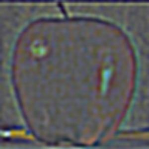
Level 3

Level 4
orange.jpeg (Gaussian Stack)

Level 0
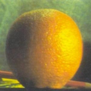
Level 1

Level 2
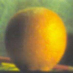
Level 3

Level 4
orange.jpeg (Laplacian Stack)
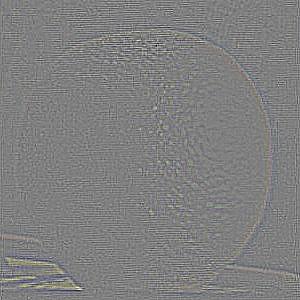
Level 0
Level 1
Level 2
Level 3

Level 4
Figure 3.42
Level 0
Level 1
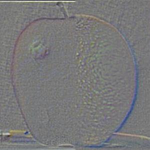
Level 2
Level 3
Level 4

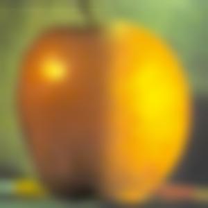
Collapsed
Part 2.4: Multiresolution Blending
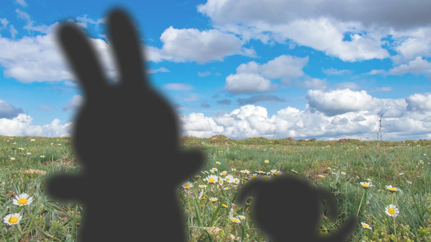
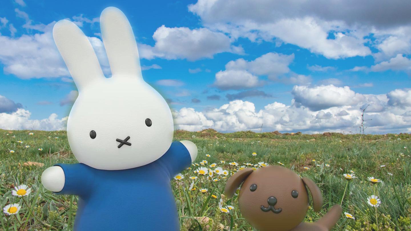
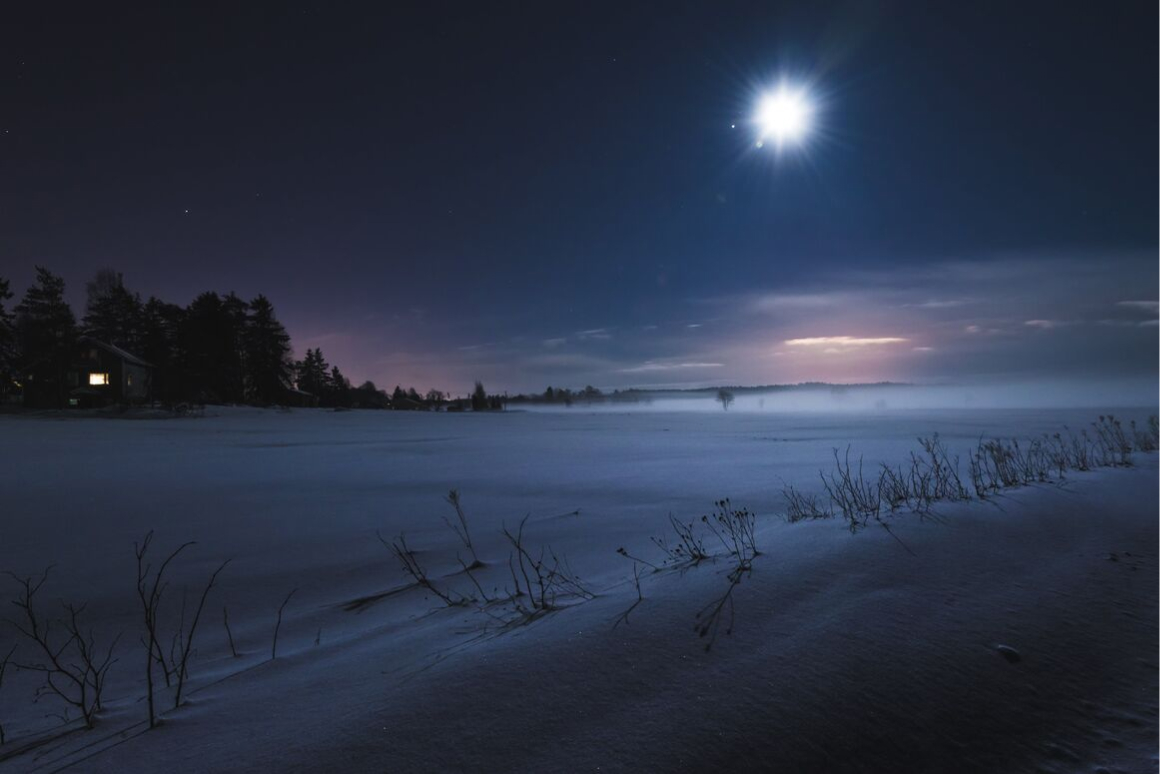
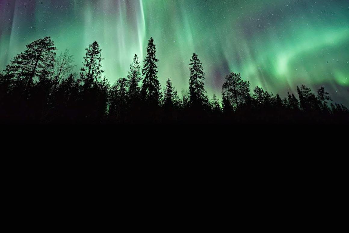
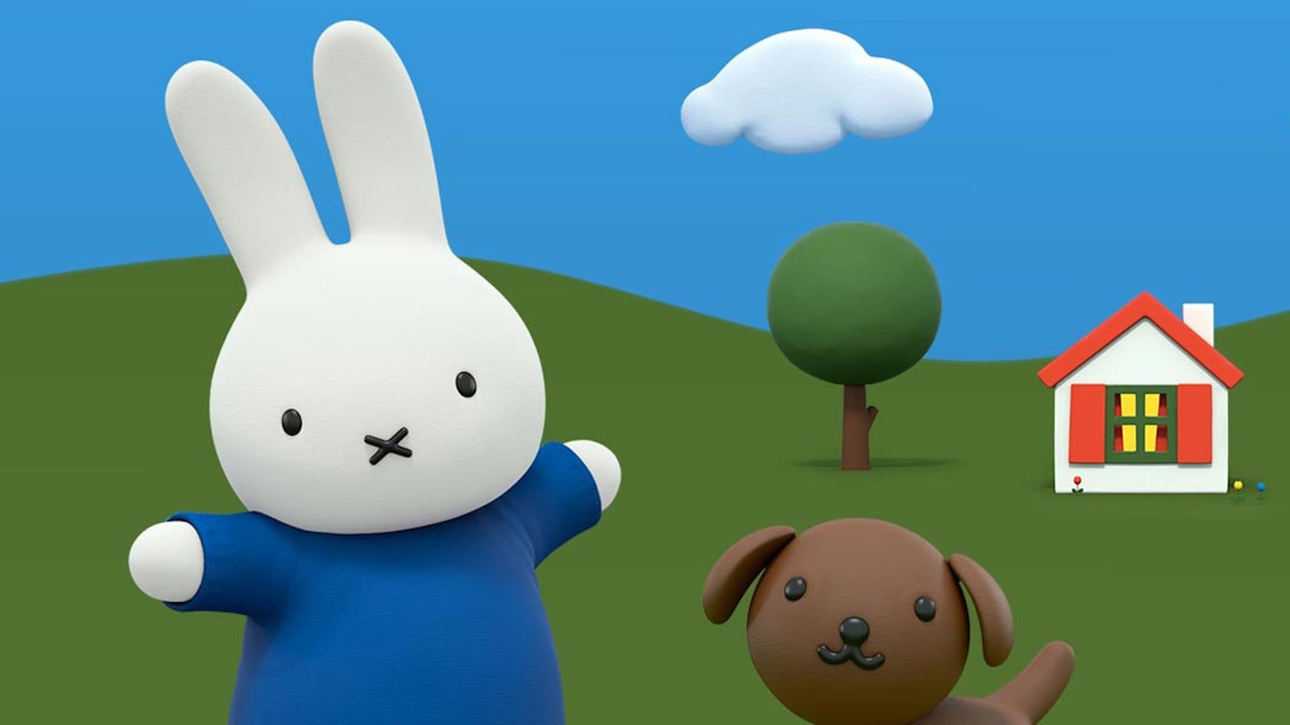
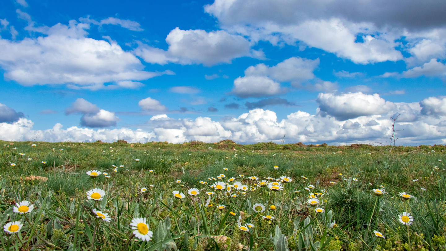
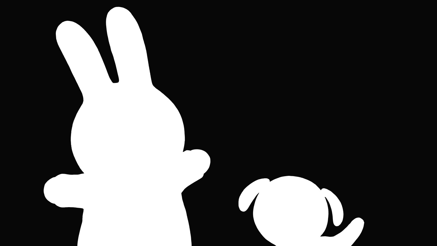
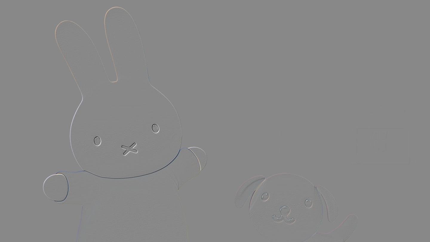
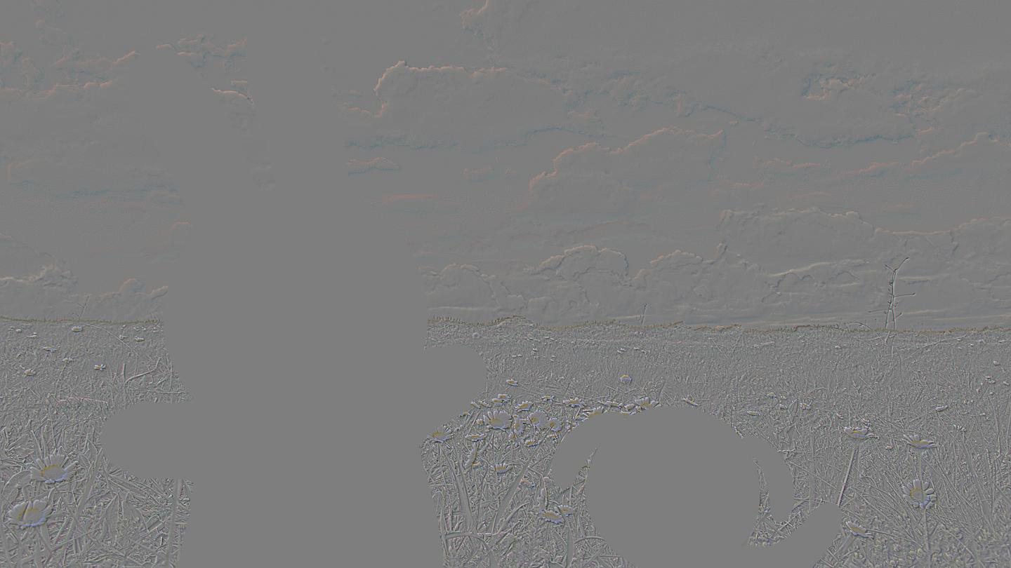
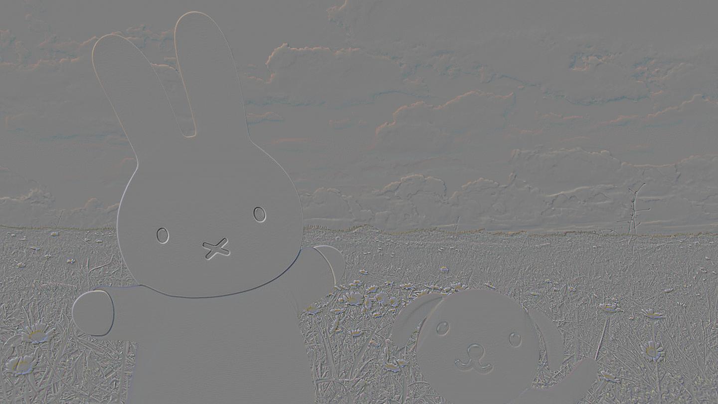
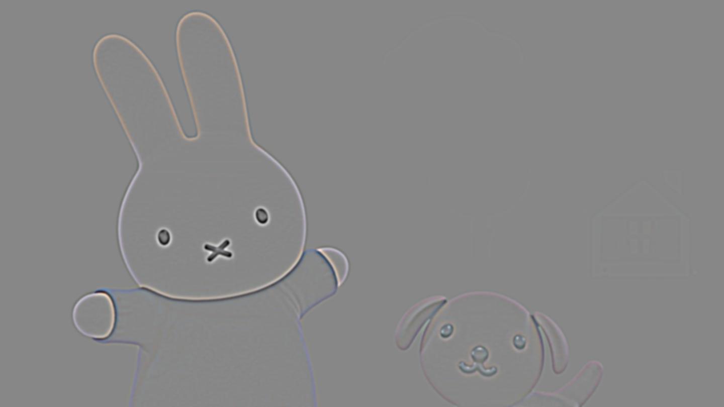
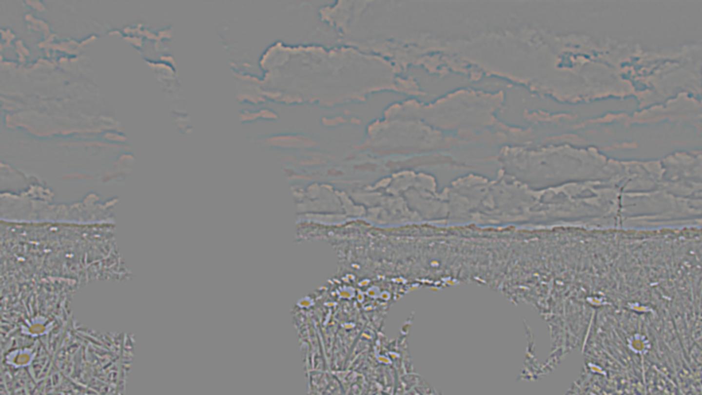
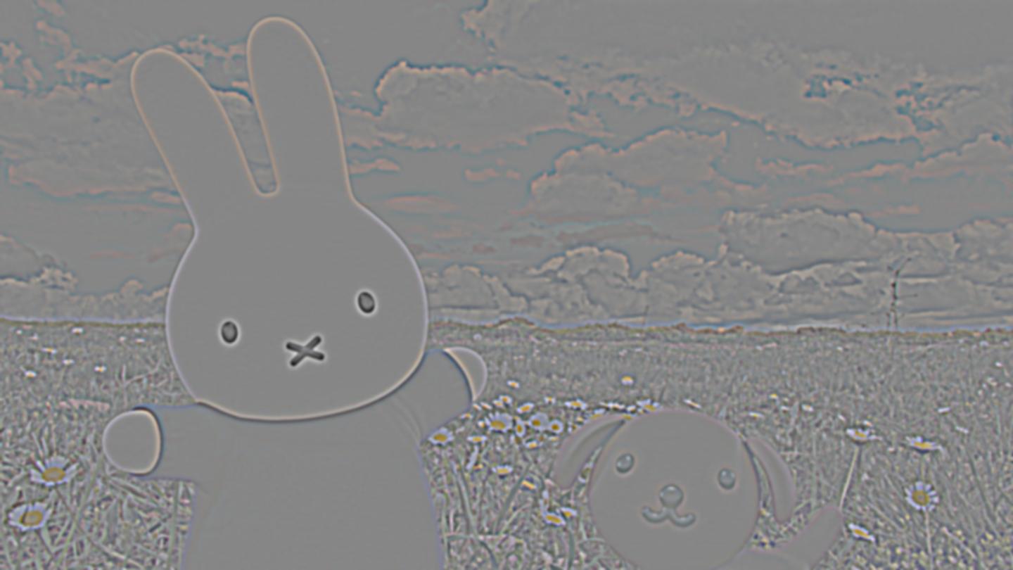
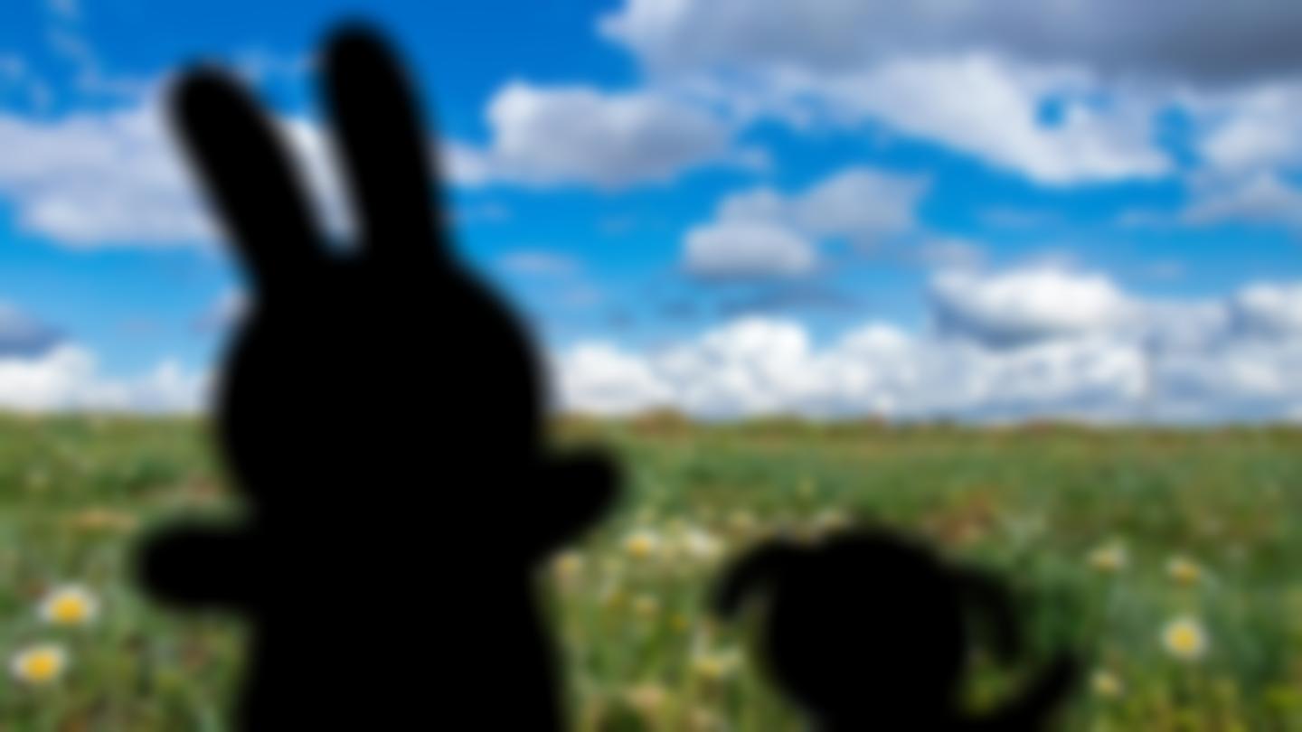
Finally, I blended some images of my own using a horizontal spline and a custom spline.
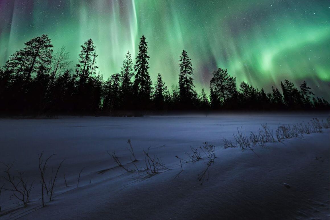
northern_lights.jpg
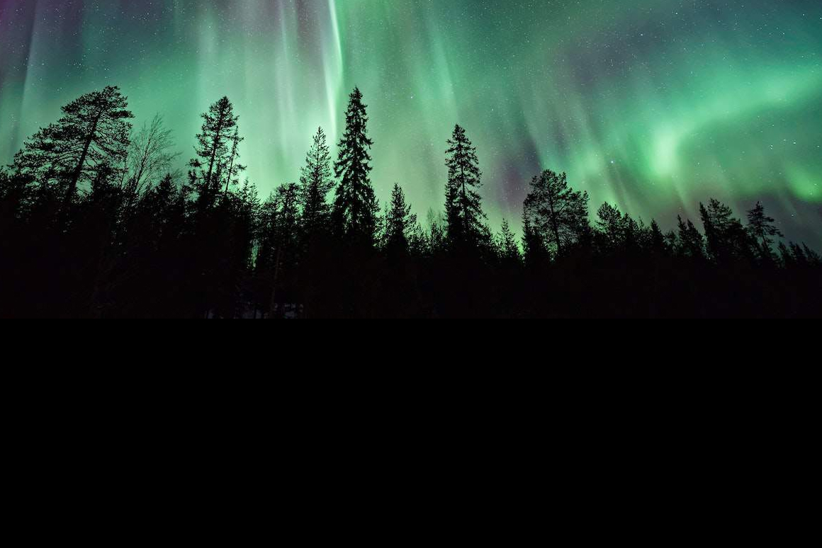
snow.jpg
Binary mask

Level 0
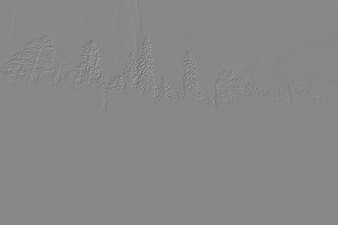
Level 2
Level 4

Collapsed


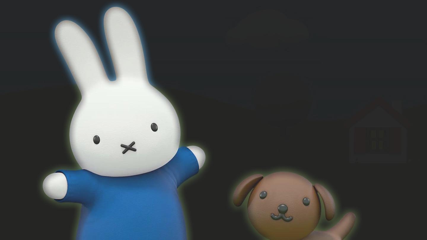
miffy.jpg
field.jpg
miffy_spline.jpg
Level 0
Level 2
Level 4

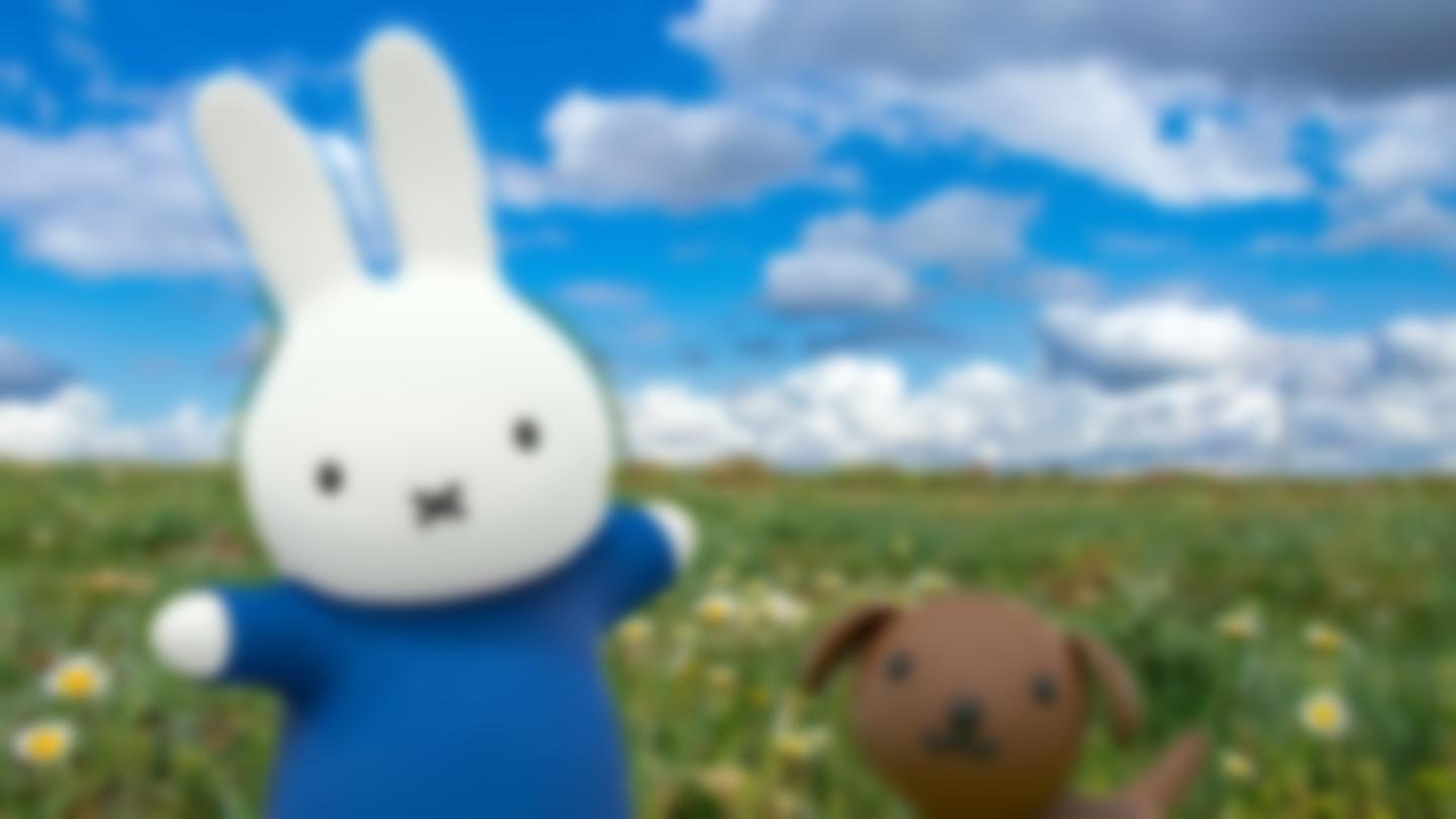
Collapsed
